Why Price Prediction Fails and What to Do Instead

The mistake described here is made by virtually every trader who tries to implement neural networks for the first time. Understanding why it fails is the prerequisite for everything that works.
The failure mode is this: take 500 days of closing prices, feed them into an LSTM, ask it to predict day 501.
In-sample, the predictions look smooth and close to actual prices. Out-of-sample, the model predicts something roughly constant or reverts to a recent mean while prices move somewhere completely different. The model appears to have learned nothing useful.
This is not a model failure. It is a data distribution failure.

neural network learns E[Y|X], the conditional expectation of Y given X. This expectation is only meaningful if the data generating distribution P(Y|X) is stable over time. If that distribution shifts, the conditional expectation the model learned from historical data no longer describes the expectation in the present.
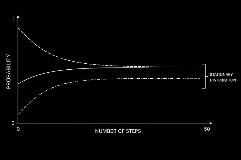
Formally, this is the problem of non-stationarity. A time series {Xₜ} is stationary if its joint distribution P(Xₜ₁, Xₜ₂, …, Xₜₙ) is invariant to time shifts. Financial price series are non-stationary in the strongest possible sense. The distribution governing equity returns in 2008 is structurally different from the distribution governing them in 2021. Mean, variance, autocorrelation, and tail behavior all shift as a function of regime, liquidity, volatility clustering, and macro conditions.
The consequence is visible in any backtest of a price-predicting neural network. The model trained on 2015 to 2019 data learns the expectation structure of that regime. When the distribution shifts in 2020, the model is fitting a moving target. Its predictions are always wrong in a systematic way that reveals it is modeling the past distribution, not the present one.
What is the solution?
Feature engineering to produce stationary or near-stationary inputs. The target variable itself should also be constructed to be approximately stationary.
For inputs, the features that have exhibited reasonable stationarity across market regimes include:
Get Retro Valix’s stories in your inbox
Join Medium for free to get updates from this writer.
Log returns over multiple windows: r_t = ln(P_t / P_{t-k}) for k in {1, 5, 20}
Volatility ratios: σ_short / σ_long where each σ is rolling realized volatility over different windows
Momentum signals normalized by volatility: r_t / σ_t, the return scaled by realized risk
Volume z-score: (V_t — μ_V) / σ_V computed over a rolling window
Spread-based signals: bid-ask spread relative to its historical distribution, or effective spread computed from trade price versus midpoint
Regime indicators: VWAP deviation, distance from rolling high and low, implied versus realized volatility ratio
For the target variable, instead of predicting next period price, predict next period direction as a binary classification problem: will the risk-adjusted return be positive? Or predict next period return z-scored against its recent distribution. Both targets are more stable than raw price or even raw return.
The practical test for whether a feature is useful: run an augmented Dickey-Fuller test on it. A p-value below 0.05 suggests the series is stationary. For features that fail this test, first-difference them or normalize by a rolling standard deviation.
Implementation note: In Python, this looks like:
from statsmodels.tsa.stattools import adfuller
import numpy as np

def check_stationarity(series, name):
    result = adfuller(series.dropna())
    print(f"{name}: ADF statistic={result[0]:.4f}, p-value={result[1]:.4f}")
    return result[1] < 0.05

# Example feature engineering
returns = df['close'].pct_change()
vol_20 = returns.rolling(20).std()
vol_5 = returns.rolling(5).std()

features = {
    'return_1d': returns,
    'return_5d': df['close'].pct_change(5),
    'vol_ratio': vol_5 / vol_20,
    'momentum': returns / vol_20,
    'volume_zscore': (df['volume'] - df['volume'].rolling(20).mean()) / df['volume'].rolling(20).std()
}

for name, series in features.items():
    is_stationary = check_stationarity(series, name)
Every feature that fails the stationarity test is a feature that will cause your model to learn the wrong distribution.
A neural network trained on your current indicator set will learn the conditional expectation of market returns given those indicators. But the conditional expectation is only as good as the features you condition on. If you had to add exactly one new feature to your model that you believe no other systematic trader is using, what would it be and why?
There is no wrong answer but there are very revealing ones.