AlexNet: The Paper That Woke Up Deep Learning

Sep 30, 2026 · Giriteka Arsène

[embed: node/0b086fea-2081]

In 2012, a neural network called AlexNet recognized photos far better than any system before it, and kick-started the deep learning boom. Here is what the paper did, what it found, and what I took away from it.

Introduction

In 2012, a single neural network cut the ImageNet error rate by almost 11 points and changed computer vision for good. The paper behind it, ImageNet Classification with Deep Convolutional Neural Networks by Alex Krizhevsky, Ilya Sutskever and Geoffrey Hinton, introduced the model now known as AlexNet.

Before 2012, most image classifiers used hand-crafted features such as SIFT or HOG, fed into a shallow classifier like an SVM. They worked on small datasets such as MNIST or CIFAR-10, but real photos vary enormously in pose, lighting and background. To learn that variety, a model needs millions of labelled images and a lot of capacity.

ImageNet supplied the data: its yearly challenge (ILSVRC) uses about 1.2 million training images across 1,000 classes, from “tabby cat” to “container ship”. The purpose of the study was to show that a large, deep convolutional neural network (CNN), trained on GPUs, could learn directly from raw pixels and beat every hand-engineered approach on this benchmark.

Procedures

AlexNet has 8 learned layers: 5 convolutional layers followed by 3 fully connected layers, ending in a 1,000-way softmax. In total it holds about 60 million parameters and 650,000 neurons. The input is a 224×224 RGB image.

Layer

What it does

Conv 1

96 kernels of 11×11×3, stride 4, then normalization and max pooling

Conv 2

256 kernels of 5×5, then normalization and max pooling

Conv 3

384 kernels of 3×3

Conv 4

384 kernels of 3×3

Conv 5

256 kernels of 3×3, then max pooling

FC 6, FC 7

4,096 neurons each, with dropout

FC 8

1,000 neurons, softmax over the classes

The size alone was not new. What made it trainable were a handful of design choices:

1. ReLU activations. Instead of tanh or sigmoid, every layer uses f(x) = max(0, x). ReLUs do not saturate, so gradients keep flowing. On CIFAR-10, a ReLU network reached 25% training error about six times faster than the same network with tanh.
2. Training on two GPUs. A GTX 580 had only 3 GB of memory, too little for the whole network. The authors split the kernels across two GPUs, which only talk to each other at certain layers.
3. Local response normalization. Each neuron’s output is scaled down by the activity of its neighbours in nearby kernel maps, a kind of “lateral inhibition”. It lowered top-1 and top-5 error by 1.4 and 1.2 points.
4. Overlapping pooling. Pooling windows of 3×3 with a stride of 2 overlap each other, unlike the usual 2×2 with stride 2. This gave a further 0.4-point gain and made the model slightly harder to overfit.

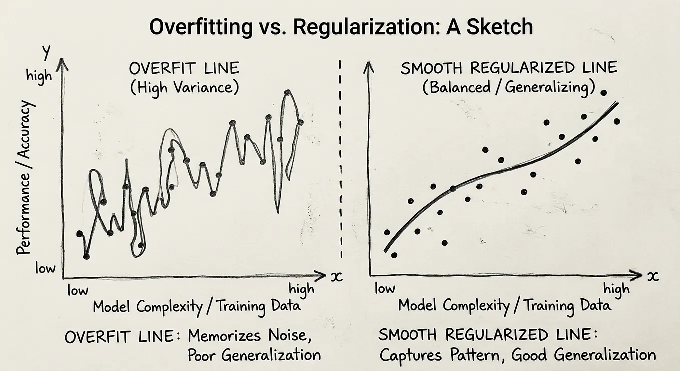
With 60 million parameters and “only” 1.2 million images, overfitting was the main danger. The authors fought it two ways:

• Data augmentation. Random 224×224 crops of the 256×256 images, plus horizontal flips, multiply the training set by 2,048. They also shifted the colours of each image along its principal components (PCA), since an object’s identity does not depend on the lighting. The colour trick alone cut top-1 error by over 1 point.
• Dropout. In the first two fully connected layers, each neuron is switched off with probability 0.5 during training. A neuron can no longer rely on specific partners, so it learns more robust features. Without dropout, the network overfit badly.

Training used stochastic gradient descent with batches of 128 images, momentum 0.9 and weight decay 0.0005. The learning rate started at 0.01 and was divided by 10 each time validation error stopped improving. Roughly 90 passes over the data took five to six days on the two GPUs.

Results

AlexNet won ILSVRC-2012 with a 15.3% top-5 error, against 26.2% for the second-best entry. Top-5 error means the right label was not among the model’s five best guesses.

Benchmark

Get Giriteka Arsène’s stories in your inbox

Join Medium for free to get updates from this writer.

Remember me for faster sign in

Model

Top-1 error

Top-5 error

ILSVRC-2012 (test)

AlexNet, 7 CNNs averaged

—

15.3%

ILSVRC-2012 (test)

Runner-up (hand-crafted features)

—

26.2%

ILSVRC-2010 (test)

AlexNet, 1 CNN

37.5%

17.0%

ILSVRC-2010 (test)

Best earlier result (SIFT + Fisher vectors)

45.7%

25.7%

A single CNN already scored 18.2% top-5 on the 2012 validation set; averaging several networks brought it down further.

The paper also looks inside the network:

• The first layer learns edge and colour detectors on its own. Kernels on one GPU became mostly colour-agnostic edge and frequency filters, while the other GPU’s kernels became colour blobs. Nobody programmed that split.
• Mistakes are reasonable. For example, a leopard photo gets “leopard” first but also “jaguar” and “cheetah”; even when the top guess is wrong, the correct label usually appears among the other four.
• The last hidden layer captures meaning. Images whose 4,096-number feature vectors are close to each other show the same kind of object, even when their pixels look nothing alike, like elephants in different poses.
• Depth matters. Removing any single middle convolutional layer raised top-1 error by about 2 points.

Conclusion

The authors conclude that a large, deep CNN trained with plain supervised learning can reach record accuracy on a very hard dataset. No hand-crafted features and no unsupervised pre-training were needed.

They stress that depth is essential: the network gets worse when any middle layer is removed. They also note that their results were limited mainly by GPU memory and training time. Bigger networks, faster GPUs and more data should simply keep improving the results.

Finally, they point to video as the next step. Motion over time gives information that still images lack, and they expected very large CNNs to use it.

Personal Notes

What struck me most is how little of AlexNet was invented from scratch. Convolutions, pooling and backpropagation already existed in LeNet-5 back in 1998. The breakthrough came from putting them together at a much larger scale, with enough data, GPUs to train on, and a few practical tricks.

This week I implemented convolution and pooling forward and backward passes in NumPy, then built LeNet-5 in Keras. That made the paper feel very concrete. For example:

• My NumPy convolution loops over every output pixel. AlexNet’s first layer alone produces 55×55×96 outputs per image, for 1.2 million images, about 90 times over. Now I understand why the authors wrote their own GPU code.
• LeNet-5 has about 60,000 parameters and reaches around 99% on MNIST in minutes. AlexNet has 1,000 times more and needed almost a week of training.

Some ideas have aged. Local response normalization was later replaced by batch normalization, and the two-GPU split was a hardware workaround. Others became standard: ReLU, dropout and data augmentation are in almost every model I have used so far.

My main takeaway is that scale and engineering matter as much as clever theory. That lesson still drives the field today, from VGG and ResNet to today’s large models.

Reference

Krizhevsky, A., Sutskever, I., & Hinton, G. E. (2012). ImageNet Classification with Deep Convolutional Neural Networks. Advances in Neural Information Processing Systems 25 (NIPS 2012).