WORKED EXAMPLES ON CAUSALITY

Jatin Madan
EXAMPLE 1: Observe Causality using CausalImpact
Let’s have a look at this with an example. Consider the following data on car drivers killed or seriously injured, and light goods drivers killed during the years 1969 to 1984 in Great Britain.

In this, we are using the CausalImpact library to estimate the causal effect of an intervention by specifying pre- and post-intervention periods and accounting for seasonality. The library employs Bayesian structural time series models to estimate the counterfactual outcome, allowing us to assess the impact of the intervention on the outcome variable.
pre_period  = [ pd.Timestamp('1969-01-01') , pd.Timestamp('1982-01-01') ]
post_period = [ pd.Timestamp('1982-02-01') , pd.Timestamp('1984-12-01') ]

ci = CausalImpact(xdat.loc[:,"car_ksi"],  pre_period, post_period,
                  nseasons=[{'period': 12}], prior_level_sd=0.05)
print(ci.summary())
## OUTPUT##
Posterior Inference {Causal Impact}
                          Average            Cumulative
Actual                    7.25               253.69
Prediction (s.d.)         7.35 (0.04)        257.37 (1.41)
95% CI                    [7.27, 7.43]       [254.52, 260.06]
Absolute effect (s.d.)    -0.1 (0.04)        -3.67 (1.41)
95% CI                    [-0.18, -0.02]     [-6.36, -0.82]
Relative effect (s.d.)    -1.43% (0.55%)     -1.43% (0.55%)
95% CI                    [-2.47%, -0.32%]   [-2.47%, -0.32%]
Posterior tail-area probability p: 0.0
Posterior prob. of a causal effect: 99.5%
Summing up the individual data points during the post-intervention
period (which can only sometimes be meaningfully interpreted), the
response variable had an overall value of 253.69. By contrast, had the intervention not taken place, we would have expected a sum of 257.37. The 95% interval of this prediction is [254.52, 260.06].
The above results are given in terms of absolute numbers. In relative
terms, the response variable showed a decrease of -1.43%. The 95%
interval of this percentage is [-2.47%, -0.32%].

This means the negative effect observed during the intervention period is statistically significant. If the experimenter had expected a positive effect, it is recommended to double-check whether anomalies in the control variables may have caused an overly optimistic expectation of what should have happened in the response variable in the absence of the intervention.
The probability of obtaining this effect by chance is very small
(Bayesian one-sided tail-area probability p = 0.0). This means the causal effect can be considered statistically significant.
EXAMPLE 2: Observe Causality using DoWhy
DoWhy is an end-to-end library for causal analysis that builds on the latest research in modeling assumptions and robustness checks. Specifically, DoWhy is organized around the four key steps that are required for any causal analysis: Model, Identify, Estimate, and Refute. The model encodes prior knowledge as a formal causal graph, identify uses graph-based methods to identify the causal effect, estimate uses statistical methods for estimating the identified estimand, and finally refute tries to refute the obtained estimate by testing the robustness of the initial model’s assumptions.
Get Jatin Madan’s stories in your inbox
Join Medium for free to get updates from this writer.
Here, we have a dataset of user spending habits over a 12-month period which includes information about each user’s signup month, their spending in each month, and whether they belong to the treatment group (i.e., whether they signed up).
## Model a causal problem
import dowhy
from dowhy import CausalModel
model = dowhy.CausalModel(data=df_i_signupmonth,
                          graph=causal_graph.replace("\n", " "),
                          treatment="treatment",
                          outcome="post_spends")
model.view_model()
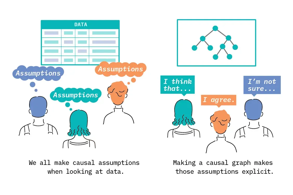
In DoWhy, a causal model is an object that encapsulates various aspects of the causal analysis process, such as the data, the treatment, the outcome, and the assumptions about the causal relationships among variables. One of the key components of the causal model in DoWhy is the causal graph, which is typically represented as a DAG.

A DAG in DoWhy is used to represent the assumed causal relationships among variables, visually displaying the structure of these relationships. The causal graph, as a DAG, is an essential input when creating an CausalModel object in DoWhy. It helps guide the identification, estimation, and refutation of causal effects.
## Identify a target estimand under the model
identified_estimand = model.identify_effect(proceed_when_unidentifiable=True)
print(identified_estimand)

##OUTPUT##
Estimand type: EstimandType.NONPARAMETRIC_ATE
### Estimand : 1
Estimand name: backdoor
Estimand expression:
     d
────────────(E[post_spends|signup_month])
d[treatment]
Estimand assumption 1, Unconfoundedness: If U→{treatment} and U→post_spends then P(post_spends|treatment,signup_month,U) = P(post_spends|treatment,signup_month)
### Estimand : 2
Estimand name: iv
Estimand expression:
 ⎡                                                             -1⎤
 ⎢       d                      ⎛       d                     ⎞  ⎥
E⎢────────────────(post_spends)⋅⎜────────────────([treatment])⎟  ⎥
 ⎣d[Z  pre_spends]              ⎝d[Z  pre_spends]             ⎠  ⎦
Estimand assumption 1, As-if-random: If U→→post_spends then ¬(U →→{Z,pre_spends})
Estimand assumption 2, Exclusion: If we remove {Z,pre_spends}→{treatment}, then ¬({Z,pre_spends}→post_spends)
### Estimand : 3
Estimand name: frontdoor
No such variable(s) found!
In this step, different causal estimands are presented for the causal effect of treatment on the outcome. Each estimand is based on a different identification strategy (backdoor, instrumental variable, or frontdoor) and relies on specific assumptions about the causal relationships among variables. These estimands represent the quantities we aim to estimate in causal analysis, given the assumed causal structure.
## Estimate causal effect based on the identified estimand
estimate = model.estimate_effect(identified_estimand,
                                 method_name='backdoor.propensity_score_matching',
                                 target_units='att')
print(estimate)

##OUTPUT##
*** Causal Estimate ***
## Identified estimand
Estimand type: EstimandType.NONPARAMETRIC_ATE
### Estimand : 1
Estimand name: backdoor
Estimand expression:
     d
────────────(E[post_spends|signup_month])
d[treatment]
Estimand assumption 1, Unconfoundedness: If U→{treatment} and U→post_spends then P(post_spends|treatment,signup_month,U) = P(post_spends|treatment,signup_month)
## Realized estimand
b: post_spends~treatment+signup_month
Target units: att
## Estimate
Mean value: 86.26916725642847
The output shows the average treatment effect on the treated (ATT) is approximately 86.27. This means that, on average, the treatment group’s post_spends increased by about 86.27 units compared to what they would have spent in the absence of the treatment.
##Refute the obtained estimate
refutation = model.refute_estimate(identified_estimand, estimate, method_name='placebo_treatment_refuter',
                     placebo_type='permute', num_simulations=20)
print(refutation)

## OUTPUT##
Refute: Use a Placebo Treatment
Estimated effect:86.26916725642847
New effect:-6.033203585751362
p value:0.22788907814083004- Estimated effect: 86.27 (original causal effect estimate)
- New effect: -6.03 (causal effect estimate with the placebo treatment)
- p-value: 0.23
The new effect of the placebo treatment is significantly different from the original estimated effect, which is a good sign. The p-value of 0.23 is greater than the standard significance level (e.g., 0.05), indicating that we cannot reject the null hypothesis that the original estimated effect is due to random chance alone.
In summary, the refutation test with the placebo treatment provides evidence that the original causal effect estimate is robust and not due to chance alone.
References
- DoWhy: An End-to-End Library for Causal Inference
- Causal Inference and Its Fundamentals
- Introduction to Causal Inference
- Time Series Causal Impact Analysis in Python
License
All code in this notebook is available as open source through the MIT license.
All text and images are free to use under the Creative Commons Attribution 3.0 license. https://creativecommons.org/licenses/by/3.0/us/
These licenses let people distribute, remix, tweak, and build upon the work, even commercially, as long as they give credit for the original creation.
Copyright 2023 AI Skunks https://github.com/aiskunks
Permission is hereby granted, free of charge, to any person obtaining a copy of this software and associated documentation files (the “Software”), to deal in the Software without restriction, including without limitation the rights to use, copy, modify, merge, publish, distribute, sublicense, and/or sell copies of the Software, and to permit persons to whom the Software is furnished to do so, subject to the following conditions:
The above copyright notice and this permission notice shall be included in all copies or substantial portions of the Software.
THE SOFTWARE IS PROVIDED “AS IS”, WITHOUT WARRANTY OF ANY KIND, EXPRESS OR IMPLIED, INCLUDING BUT NOT LIMITED TO THE WARRANTIES OF MERCHANTABILITY, FITNESS FOR A PARTICULAR PURPOSE AND NONINFRINGEMENT. IN NO EVENT SHALL THE AUTHORS OR COPYRIGHT HOLDERS BE LIABLE FOR ANY CLAIM, DAMAGES OR OTHER LIABILITY, WHETHER IN AN ACTION OF CONTRACT, TORT OR OTHERWISE, ARISING FROM, OUT OF OR IN CONNECTION WITH THE SOFTWARE OR THE USE OR OTHER DEALINGS IN THE SOFTWARE.