Logistic Regression from Scratch

Figure 1

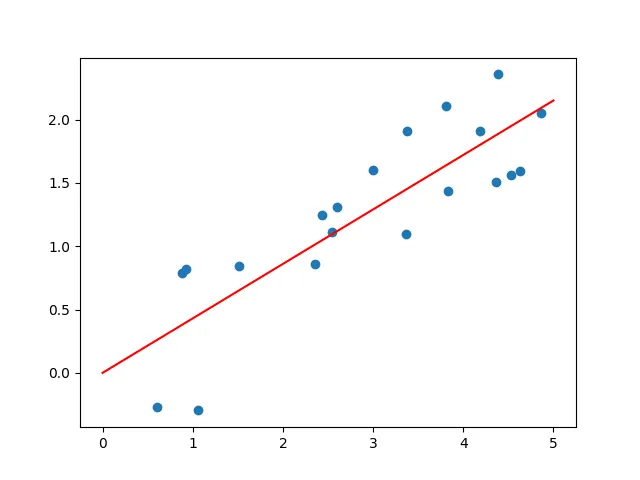
I’ve finally gotten around to the second post in my series “Machine Learning from Scratch.” In the previous post, I tackled linear regression. Here I will discuss a method of classifying data known as logistic regression. Just as in linear regression, our inputs are n-dimensional data points (vectors). Our outputs are discrete numerical values (classes) to which a given data point belongs. For logistic regression we consider binary classification problems: that is, there are only 2 classes into which each data point could fall.

Note: throughout this post, I will be using “numpy notation” to supplement standard mathematical notation, meaning that a scalar operation applied to a vector is understood as applying that operation elementwise. This simplifies some expressions.

As in linear regression, we start with a model defined by a vector of numerical parameters β which maps a data point x to a result via

If we have multiple data points we can construct a matrix X by arranging them in rows, with each row representing one datapoint. We can then compute the results for all of them at once by matrix multiplication.

This was all discussed in the previous post if you need a refresher.

The model’s output for the ith datapoint, which we will denote z_i, is calculated as

or in index form with no explicit vectors

Equation 1

How can this model be used for splitting data into two categories?

Note that the equation x * β = 0 defines a line, plane, or hyperplane depending on whether x and β have 2, 3, or more dimensions. So one way we could classify data is to say that everything falling on one side of this hyperplane (e.g. x * β < 0) will be placed in one class, and everything falling on the other side (x * β > 0) will be placed in the other.

The hyperplane becomes a “classification boundary” dividing the data into two categories, as seen in Figure 1. This type of model is called a linear classifier.

The Scenario

I will be building a linear classifier for the “Titanic — Machine Learning from Disaster” Kaggle competition. In this competition, there is a table of training data containing information about the passengers of the Titanic — age, sex, ticket price, etc. It also includes a column indicating whether that passenger survived (1) or did not survive (0). The goal is to predict this column by looking at the other data. This is a binary classification problem.

Let’s take a look at the data.

train_data = pd.read_csv('/kaggle/input/competitions/titanic/train.csv')
train_data.head()

Figure 2

What are the Odds?

Another way we could look at this task is to build a model which takes a vector of data for a passenger and spits out a probability of survival. Then we could predict that the passenger survived if the probability is greater than a cutoff value, say 50%. We want to find a way for our model output z_i defined by Equation 1 to be interpreted this way.

The problem with this is that z_i can range from -∞ to ∞. How do we interpret it as a probability between 0 and 1? The key is a concept called odds. If we have two probabilities p and q, we may consider the odds ratio p/q. This expresses how likely p is compared to q.

Given our Titanic problem, if the probability of survival is p, and the probability of death is 1 — p, then the odds in favor of survival are p/(1 — p). Notice that for p = 0.5, the odds are 1 (i.e. death and survival are equally likely). For p = 0, the odds are 0 (survival is impossible). As p → 1, the odds approach infinity, expressing that the likelihood of survival grows without bound. This seems promising, but the odds still cannot be a negative number.

We can instead consider the log odds: log(p/(1-p)). This quantity is also called a logit. It has a range from -∞ to ∞, which is exactly what we want. We will treat our model’s outputs z_i as logits and then convert them into probabilities. To do this, we need to invert the log-odds formula.

Let

Then

We have now obtained the standard logistic or sigmoid function:

Hence the name “logistic regression.” This functions converts the logits z_i output by the model into probabilities. Additionally, a logit of 0 corresponds to a probability of 0.5. Thus, the classification boundary x * β = 0 discussed earlier represents using logits and classifying every data point based on whether the predicted probability of survival is greater or less than 50%.

Maximum Likelihood Estimation

The question now is how to fit this linear model so that it best represents our data. We will do this using a technique called Maximum Likelihood Estimation (MLE). It involves choosing a probability distribution with variable parameters which could have generated the observed data, then finding the values of the parameters which would make the observed data most likely.

What probability distribution will we choose? We can hypothesize a binomial distribution where there is a fixed probability p_i of the ith passenger surviving. These probabilities will be generated by our model via

Equation 2

Based on Equation 1, p_i depends both on the data about each passenger, X_i, and the model parameters β.

If we have a vector y of observed survivals (y_i = 1 means the ith passenger survived, and y_i = 0 means they didn’t), the likelihood of the observed survivals given survival probabilities p_i is

Note we are assuming each passenger’s probability of survival is independent of everyone else’s.

To make this expression easier to work with, we can take it’s logarithm, which gives us the log likelihood:

Rather than maximizing this, it is a common convention to minimize the negative log-likelihood, or “loss function.” This will be familiar from the post about linear regression, where the loss function was Mean Squared Error.

Here, the loss is

Psst…this is called “Binary Cross-Entropy” loss. Check it out.

Using Equation 2 the loss becomes

Equation 3

Unlike in the case of linear regression, there is no closed-form solution to find the minimum of this function so we need to rely on approximation methods.

Minimizing loss by gradient descent

Even in relatively simple scenarios like this one, finding the exact minimum of a loss function is intractable. Imagine how difficult it must be in more complex situations. We need some way to handle this. The method explained here is by far one of the most important techniques in machine learning: gradient descent. Along with backpropagation (which I will cover in a future post), it is one of the fundamental mechanisms used to train neural networks.

The core idea is actually very simple. If we want to find the minimum of a function, we could just take a step “downhill” — in the direction opposite of the function’s slope. The slope of a function is its derivative, or if we’re in multiple dimensions, its gradient. So gradient descent means we step in the direction of the negative gradient of the function. Then, we compute the gradient at our new location and do it again, continuing until some specified stopping condition is reached.

Get Perrin Alaine-Sedano’s stories in your inbox

Join Medium for free to get updates from this writer.

Remember me for faster sign in

During each update step, we will adjust our model parameters in the direction of the negative gradient of the loss w.r.t. these parameters. However, we need to decide how far to step downhill each time, which we will do by multiplying a value η by the gradient, called the learning rate. Thus, the adjustment Δ to the model parameters at each step is given by the following equation:

Figure 3. A single step of gradient descent visualized. Graph created with Desmos.

Now let’s compute the derivative of the loss function from Equation 3 w.r.t. a single model parameter β_i

By repeated application of the chain rule, this becomes

Expression 1

Here’s a helpful fun fact.

The proof is left as an exercise to Wikipedia.

So Expression 1 reduces to

Expression 2

Based on Equation 1,

so

The right hand side terms will be zero except when k = i, so we get

Expression 2 now becomes

This looks like the ith term of a dot product between X^T and the vector σ(z) — y. Since the gradient w.r.t. β is just a vector of the derivatives for each β_i, it will be

Equation 4

Phew!

Now that we’ve gotten that out of the way, it’s time to tackle the Titanic.

Application

I will use three columns from Figure 2 as my data points, converting the ‘Sex’ column to numerical values

predictors = df[['Pclass', 'Sex', 'Age']]
predictors.loc[predictors.Sex == 'male', 'Sex'] = 0
predictors.loc[predictors.Sex == 'female', 'Sex'] = 1

Then I convert this table into a numpy array and add a column of 1s to facilitate a bias term (discussed in the prior tutorial on linear regression). Without this, if all three predictor variables were zero, the logit output by the model would have to be zero no matter what. This is clearly undesirable.

x = predictors.to_numpy(dtype=np.float64, na_value=0)
x = np.hstack((x, np.ones((x.shape[0], 1))))

Finally I’ll get the actual data about who survived.

predictee = train_data['Survived']
y = predictee.to_numpy(dtype=np.float64, na_value=0)

Then let’s define the model:

model = np.random.uniform(size=4)

The parameters are initialized randomly.

We need some helper functions.

# Logistic function
def sigmoid(x):
    return 1/(1+np.exp(-x))

# Binary Cross Entropy averaged over the training examples
def cross_entropy_loss(x, y):
    return ((1 - y) @ x + np.sum(np.log(1 + np.exp(-x)))) / y.size

# Negative gradient of BCE averaged over training examples
def negative_grad_ce_loss(x, y, logits):
    return x.transpose() @ (y - sigmoid(logits)) / y.size

These are all based on the equations shown earlier, with loss and its gradient being divided by the number of data points to get the average. I found that without doing this, the calculations became riddled with infinities due to overflow in np.exp.

You may notice that the form of the cross-entropy loss is different than the one presented in Equation 3, but it is equivalent:

Now we can run the training loop, adjusting the model repeatedly by gradient descent for a large number of steps.

# Parameters
num_steps = 4000
learning_rate = 0.005

# plotting
training_steps = np.linspace(0, num_steps, num_steps)
accuracies = []
losses = []

# Training loop
for i in range(num_steps):
    logits = x @ model
    loss = cross_entropy_loss(logits, y)
    model += learning_rate * negative_grad_ce_loss(x, y, logits)

    losses.append(loss)
    
    # get accuracy
    predictions = np.round(sigmoid(logits)).astype(np.int64)
    accuracies.append(np.sum(predictions == y) / y.size)

These plots show loss and accuracy for the model over all the training steps (with perfect accuracy being 1).

Figure 4

Figure 5

As you can see, there is quite a bit of improvement, although most of it happens in the beginning. Diminishing returns is a common phenomenon in both human and machine learning.

The latest accuracy my model obtained for the Kaggle competition is 77%. Not great, but certainly much better than random guessing. I’m sure there are many improvements I could make, but my goal here was just to demonstrate the basics of logistic regression.

Conclusion

And that’s it for logistic regression! In the next tutorial, we’ll take things further and see how the ideas developed here form the backbone of neural networks. See you next time!

The code is available on Kaggle.