Uninformed Search Algorithms, also called Blind Search Algorithms, are search methods that find a solution using only the problem's initial state, available actions and goal state, without any additional guidance or heuristic information.
- Use only the initial state, available actions and goal state to find a solution.
- Do not rely on heuristic information or prior knowledge.
- Explore the search space in a systematic manner.
- Commonly applied in pathfinding, puzzle-solving and state-space search problems.
- Can be less efficient because many unnecessary states may be explored before reaching the goal.
Types of Uninformed Search Algorithms
1. Breadth-First Search (BFS)
Breadth-First Search is an uninformed search algorithm that explores nodes level by level. It visits all nodes at the current depth before moving to the next depth level and uses a Queue (FIFO) to manage the search process.
- The bfs() function uses Breadth-First Search (BFS) to find the shortest path in a 2D maze.
- It explores neighboring cells level by level using a queue (FIFO) and avoids revisiting cells with a visited set.
- When the goal is reached, the function returns the complete path from the start to the goal.
- The visualize_maze() function uses Matplotlib to display the maze, highlighting the start position, goal position, and the path found by BFS.
- imshow() is used to draw the maze, while scatter() marks important positions and the solution path.
import numpy as np
import matplotlib.pyplot as plt
from matplotlib.colors import ListedColormap
from collections import deque

def bfs(maze, start, goal):
    queue = deque([(start, [])])
    visited = set()

    while queue:
        current, path = queue.popleft()
        x, y = current

        if current == goal:
            return path + [current]

        if current in visited:
            continue

        visited.add(current)

        for dx, dy in [(0, 1), (0, -1), (1, 0), (-1, 0)]:
            nx, ny = x + dx, y + dy
            if 0 <= nx < len(maze) and 0 <= ny < len(maze[0]) and maze[nx][ny] != 1:
                queue.append(((nx, ny), path + [current]))

    return None

def visualize_maze(maze, start, goal, path=None):
    cmap = ListedColormap(['white', 'black', 'red', 'blue', 'green'])
    bounds = [0, 0.5, 1.5, 2.5, 3.5, 4.5]
    norm = plt.Normalize(bounds[0], bounds[-1])

    fig, ax = plt.subplots()
    ax.imshow(maze, cmap=cmap, norm=norm)

    ax.scatter(start[1], start[0], color='yellow', marker='o', label='Start')
    ax.scatter(goal[1], goal[0], color='purple', marker='o', label='Goal')

    if path:
        for node in path[1:-1]:
            ax.scatter(node[1], node[0], color='green', marker='o')

    ax.legend()
    plt.show()

maze = np.array([
    [0, 0, 0, 0, 0],
    [1, 1, 0, 1, 1],
    [0, 0, 0, 0, 0],
    [0, 1, 1, 1, 0],
    [0, 0, 0, 0, 0]
])

start = (0, 0)
goal = (4, 4)

path = bfs(maze, start, goal)

visualize_maze(maze, start, goal, path)
Output:
.png)
2. Depth-First Search (DFS)
Depth-First Search (DFS) is an uninformed search algorithm that explores one path as deeply as possible before backtracking. It uses a Stack (LIFO) to keep track of nodes during the search.
- The dfs() function uses Depth-First Search (DFS) to find a path in a 2D maze.
- It explores one path as deeply as possible using a stack (LIFO) and avoids revisiting cells with a visited set.
- When the goal is reached, the function returns the path from the start to the goal.
- The visualize_maze() function uses Matplotlib to display the maze, highlighting the start position, goal position and the path found by DFS.
- imshow() is used to draw the maze, while scatter() marks important positions and the solution path.
def visualize_maze(maze, start, goal, path=None):
    cmap = ListedColormap(['white', 'black', 'red', 'blue', 'green'])
    bounds = [0, 0.5, 1.5, 2.5, 3.5, 4.5]
    norm = plt.Normalize(bounds[0], bounds[-1])

    fig, ax = plt.subplots()
    ax.imshow(maze, cmap=cmap, norm=norm)

    ax.scatter(start[1], start[0], color='yellow', marker='o', label='Start')
    ax.scatter(goal[1], goal[0], color='purple', marker='o', label='Goal')

    if path:
        for node in path[1:-1]:
            ax.scatter(node[1], node[0], color='green', marker='o')

    ax.legend()
    plt.show()

def dfs(maze, start, goal):
    stack = [(start, [])]
    visited = set()

    while stack:
        current, path = stack.pop()
        x, y = current

        if current == goal:
            return path + [current]

        if current in visited:
            continue

        visited.add(current)

        for dx, dy in [(0, 1), (0, -1), (1, 0), (-1, 0)]:
            nx, ny = x + dx, y + dy
            if 0 <= nx < len(maze) and 0 <= ny < len(maze[0]) and maze[nx][ny] != 1:
                stack.append(((nx, ny), path + [current]))

    return None

maze = np.array([
    [0, 0, 0, 0, 0],
    [1, 1, 0, 1, 1],
    [0, 0, 0, 0, 0],
    [0, 1, 1, 1, 0],
    [0, 0, 0, 0, 0]
])

start = (0, 0)
goal = (4, 4)

path = dfs(maze, start, goal)

visualize_maze(maze, start, goal, path)
Output:
.png)
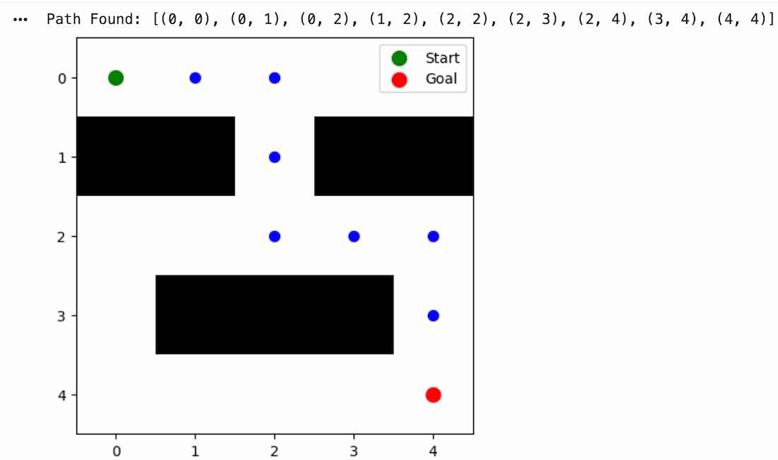
3. Depth-Limited Search (DLS)
Depth Limited Search (DLS) is a variation of Depth-First Search (DFS) that restricts the search to a predefined depth limit. This helps prevent infinite exploration in large or infinite search spaces.
- The dls() function uses Depth-Limited Search (DLS) to find a path in a 2D maze within a specified depth limit.
- It explores nodes in a depth-first manner and stops when the depth limit is reached.
- A visited set prevents revisiting cells during the search.
- If the goal is found, the function returns the path; otherwise, it returns None.
- The visualize_maze() function uses Matplotlib to display the maze and the path found by DLS.
import numpy as np
import matplotlib.pyplot as plt
from collections import deque

def dls(maze, start, goal, limit):
    stack = [(start, [start], 0)]
    visited = set()

    while stack:
        current, path, depth = stack.pop()

        if current == goal:
            return path

        if depth >= limit:
            continue

        if current in visited:
            continue

        visited.add(current)

        x, y = current

        for dx, dy in [(0, 1), (0, -1), (1, 0), (-1, 0)]:
            nx, ny = x + dx, y + dy

            if (
                0 <= nx < len(maze)
                and 0 <= ny < len(maze[0])
                and maze[nx][ny] != 1
            ):
                stack.append(((nx, ny), path + [(nx, ny)], depth + 1))

    return None


def visualize_maze(maze, start, goal, path=None):
    plt.figure(figsize=(5, 5))
    plt.imshow(maze, cmap="binary")

    plt.scatter(start[1], start[0], color="green", s=100, label="Start")
    plt.scatter(goal[1], goal[0], color="red", s=100, label="Goal")

    if path:
        for x, y in path[1:-1]:
            plt.scatter(y, x, color="blue", s=50)

    plt.legend()
    plt.show()

maze = np.array([
    [0, 0, 0, 0, 0],
    [1, 1, 0, 1, 1],
    [0, 0, 0, 0, 0],
    [0, 1, 1, 1, 0],
    [0, 0, 0, 0, 0]
])

start = (0, 0)
goal = (4, 4)
depth_limit = 10

path = dls(maze, start, goal, depth_limit)

if path:
    print("Path Found:", path)
else:
    print("No Path Found within Depth Limit")

visualize_maze(maze, start, goal, path)
Output:
4. Iterative Deepening Depth-First Search (IDDFS)
Iterative Deepening Depth-First Search (IDDFS) combines the advantages of BFS and DFS by repeatedly performing Depth-First Search with increasing depth limits until the goal is found.
- The iddfs() function uses Iterative Deepening Depth-First Search (IDDFS) to find a path in a 2D maze.
- It repeatedly performs Depth-Limited Search (DLS) with increasing depth limits until the goal is found.
- This combines the low memory usage of DFS with the completeness of BFS.
- If the goal is found, the function returns the path; otherwise, it returns None.
- The visualize_maze() function uses Matplotlib to display the maze and the path found by IDDFS.

The IDDFS algorithm successfully found a path from the start node to the goal node by gradually increasing the search depth while avoiding obstacles.
5. Uniform-Cost Search (UCS)
Uniform-Cost Search (UCS) is an uninformed search algorithm that expands the node with the lowest path cost first. Unlike BFS, it considers the cost of reaching each node and guarantees the optimal path when all costs are non-negative.
- The uniform_cost_search() function finds the least-cost path in a weighted graph.
- It uses a priority queue to always explore the lowest-cost node first.
- If the goal is reached, the function returns the optimal path.
- The visualize_graph() function displays the graph and highlights the path found by UCS.
import networkx as nx
import matplotlib.pyplot as plt
import heapq

class Node:
    def __init__(self, state, parent=None, action=None, path_cost=0):
        self.state = state
        self.parent = parent
        self.action = action
        self.path_cost = path_cost

    def __lt__(self, other):
        return self.path_cost < other.path_cost

def uniform_cost_search(graph, start, goal):
    frontier = []
    heapq.heappush(frontier, Node(start))
    explored = set()
    path = []

    while frontier:
        node = heapq.heappop(frontier)

        if node.state == goal:
            path = reconstruct_path(node)
            break

        explored.add(node.state)

        for (cost, result_state) in graph[node.state]:
            if result_state not in explored:
                child_cost = node.path_cost + cost
                child_node = Node(result_state, node, None, child_cost)
                if not any(frontier_node.state == result_state and
                           frontier_node.path_cost <= child_cost for frontier_node in frontier):
                    heapq.heappush(frontier, child_node)

    return path

def reconstruct_path(node):
    path = []
    while node:
        path.append(node.state)
        node = node.parent
    return path[::-1]

def visualize_graph(graph, path=None):
    G = nx.DiGraph()
    labels = {}
    for node, edges in graph.items():
        for cost, child_node in edges:
            G.add_edge(node, child_node, weight=cost)
            labels[(node, child_node)] = cost

    pos = nx.spring_layout(G)
    nx.draw(G, pos, with_labels=True, node_color='lightblue', node_size=2000)
    nx.draw_networkx_edge_labels(G, pos, edge_labels=labels)

    if path:
        path_edges = list(zip(path[:-1], path[1:]))
        nx.draw_networkx_edges(G, pos, edgelist=path_edges, edge_color='r', width=2)

    plt.show()

graph = {
    'A': [(1, 'B'), (3, 'C')],
    'B': [(2, 'D')],
    'C': [(5, 'D'), (2, 'B')],
    'D': []
}

start = 'A'
goal = 'D'
path = uniform_cost_search(graph, start, goal)

visualize_graph(graph, path)
print("Path from", start, "to", goal, ":", path)
Output:
Path from A to D : ['A', 'B', 'D']
.png)
Download complete code from here
Applications
- Used in navigation systems and robotics to find paths between locations.
- Helps solve puzzles such as the Eight Puzzle and Fifteen Puzzle by finding a sequence of valid moves.
- Supports game AI by exploring possible moves and strategies.
- Assists robots in planning routes while avoiding obstacles.
- Used in web crawling to systematically discover and index web pages through links.
Limitations
- May explore many unnecessary states before finding a solution.
- Can be slow and inefficient for large or complex search spaces.
- Some algorithms do not guarantee the shortest or optimal solution.
- Often require high memory or computational resources as the search space grows.
- Performance decreases significantly when the number of possible states is very large.