Transformers Explained: Why Attention Is Truly All You Need

In 2017, “Attention Is All You Need” introduced the Transformer architecture that replaced RNNs and LSTMs as the backbone of modern AI. This article provides a clear, step-by-step explanation of why it still dominates in 2026. We expose RNN limitations — sequential processing and vanishing gradients — then explore every core component: token embeddings, sinusoidal positional encodings, scaled dot-product self-attention, multi-head attention, masked self-attention, cross-attention, feed-forward networks, residuals, and layer normalization. Perfect for beginners and experts alike, this guide reveals how attention unlocked full parallelization and effortless long-range dependencies, proving it truly was all you need.

If you’re not a Medium subscriber, click here to read the full article.

1. Why Transformers? The Fundamental Limitations of RNNs and LSTMs

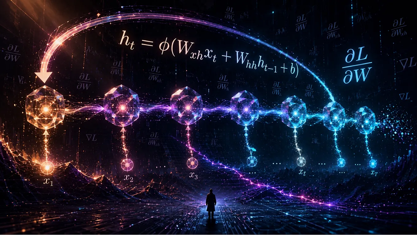
Before Transformers, Recurrent Neural Networks (RNNs) and Long Short-Term Memory (LSTMs) dominated NLP. These models processed tokens sequentially, maintaining a hidden state that evolved step-by-step.

Major issues:

• Sequential dependency: Tokens are processed one at a time → training cannot be parallelized efficiently. On large datasets, this made training painfully slow.
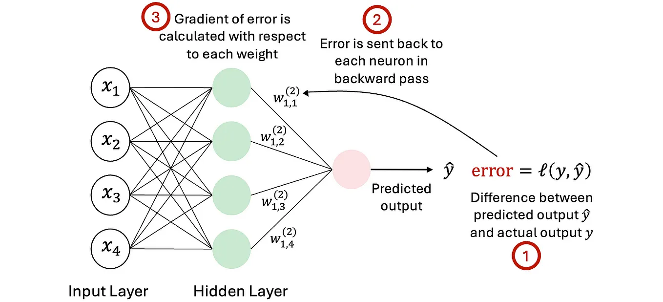
• Vanishing and exploding gradients: As sequences grew longer (e.g., >50 tokens), gradients during backpropagation through time would shrink to near zero or explode, destroying the model’s ability to learn long-range dependencies (e.g., connecting “it” to “animal” across many words).

Transformers solve both by letting every token attend to all other tokens simultaneously — no recurrence, no sequential bottleneck. The entire sequence is processed in parallel, capturing global context instantly.

2. Overview of Transformer Architecture

A standard Transformer consists of two stacks of identical layers (N = 6 in the original paper, often 12+ in modern models):

• Encoder Stack (N layers): Reads the input sequence and builds rich contextual representations.
• Decoder Stack (N layers): Generates the output sequence autoregressively, using both its own previous outputs and the encoder’s representations.

The encoder produces a fixed set of contextual vectors; the decoder “queries” them at every step.

Information flow:

1. Input tokens are embedded into dense vectors and Positional encodings are added to preserve order.
2. The encoder applies self-attention and feed-forward networks.
3. The decoder uses masked self-attention, cross-attention, and feed-forward networks.
4. Final output is projected to vocabulary probabilities via linear and softmax layers.

Each layer includes residual connections and layer normalization for stability.

3. Input Processing: Embeddings and Positional Encoding

3.1 Token Emdeddings

Text inputs are first tokenized (e.g., into words or subwords) and then each token is mapped to a dense vector of dimension d or d_model​ (original = 512). Basically, embeddings capturing semantic meaning, such as “The cat ate the mouse” becoming vectors like [0.21, -0.13, 0.87, …] for each token. For a sequence of length n (max 256 in the 2017 model):

E ∈ ℝ^{n × d}

Transformers have no inherent notion of order because self-attention is permutation-invariant. Without positional information, “the cat chased the mouse” and “the mouse chased the cat” would be indistinguishable.

3.2 Positional Encoding

To address this, positional encodings (PE) are added to inject sequence order information. The original paper uses sinusoidal functions.

For position pos and dimension i:

These are added element-wise to the token embeddings:

X = E + PE

These distinct vectors in X ensure that the model can differentiate positional contexts.

The sinusoidal design enables extrapolation to longer sequences than seen during training and encodes periodicity, helping with patterns like sentence structure.

Visualizing positional encoding:

erdem.pl

An example for a small embedding dimension d = 4. The positions 0 to 3 illustrates the uniqueness:

• Position 0: [sin(0/1000⁰), cos(0/10000⁰), sin(0/10000^{2/4}), cos(0/10000^{2/4})] ≈ [0, 1, 0, 1]
• Position 1: ≈ [0.84, 0.54, 0.01, 1.0]
• Position 2: ≈ [0.91, -0.43, 0.02, 1.0]
• Position 3: ≈ [0.14, -0.99, 0.03, 1.0]

Key advantages:

• Periodic & continuous → natural extrapolation to longer sequences.
• Linear combinations of sines/cosines encode relative positions.
• Bounded [-1, 1] → matches normalized embeddings.
• Zero extra parameters → reduces overfitting risk.

4. The Heart: Scaled Dot-Product Self-Attention

Self-attention computes weighted representations by allowing each token to attend to all others, determining “how important is that word for understanding me?” To achieve self-attention, input X is linearly projected to three matrices of Queries (Q), Keys (K), and Values (V):

where W^Q , W^K and W^V are learnable weight matrices to project input sequence X to Q, K, V matrices. Additionally, n is the length of the input sequence, d is the dimension of the input embeddings. Their matrix representation are given as below:

Attention scores: The model calculates how much each token should attend to every other token using scaled dot-products:

The 1/√dₖ ​​​​ scaling prevents dot products from growing too large in high dimensions, stabilizing softmax gradients.

Softmax Normalization: The raw scores are passed through a softmax to obtain probabilities as attention weights (heatmap):

Attention Output: The final output is a weighted sum of the values:

The result is Z: a new matrix where every token now contains the
weighted context of the entire sequence.

Here is visualization of the Self-Attention:

The overall scaled-dot-product self-attention can be represented in matrix form:

This mechanism excels at capturing long-range dependencies without regard to positional distance.

Intuitive examples:

• “the cat chased the mouse” → high attention from “chased” to “cat”.
• “The animal didn’t cross the street because it was tired” → “it” attends strongly to “animal”, not “street”.

This captures long-range dependencies regardless of distance.

5. Multi-Head Attention — Multiple Perspectives

To capture different types of relationships simultaneously, self-attention runs in parallel across multiple “heads.” Each head learns to focus on different aspects :

• Head 1: Grammatical relationships.
• Head 2: Action-Object connections.
• Head 3: Entity recognition.

To achieve multi-head self-attention, the input X is projected into multiple sets of queries, keys, and values, each corresponding to a different attention head.

For each head i:

Concatenate and project:

Each head specializes: one on syntax, one on semantics, one on coreference, etc. This dramatically increases representational power.

Get LM Po’s stories in your inbox

Join Medium for free to get updates from this writer.

Remember me for faster sign in

A summary visual representation of multi-head attention with h heads is shown below:

6. Position-wise Feed-Forward Networks (FFNs)

After every attention sub-layer, a two-layer Multi-Layer Perceptron (MLP) is applied independently to each token. This is an expand-and-compress architecture. It projects the data into a much higher dimension (dff​=2048, a 4x expansion from 512) to extract complex features via a ReLU activation, before compressing it back down to the original 512 dimensions.

Modern variants (BERT, GPT) use GELU instead of ReLU for smoother gradients and better performance with LayerNorm. This adds non-linearity and allows token-specific transformations beyond attention.

7. Residual Connections & Layer Normalization

Deep neural networks famously struggle to train due to vanishing gradients. Transformers solve this with two ubiquitous mechanisms that wrap around the attention and FFN blocks described above.

• Residual Connections: Shortcut paths that bypass sub-layers, allowing gradients to flow unimpeded through stacks of 100+ layers.

• Layer Normalization (LayerNorm): Normalizes output per-token across all features, stabilizing learning times and handling variable sequence lengths flawlessly. LayerNorm formula:

where μ and σ² computed over the d features of a single token.

Residual connections provide shortcut paths for gradients → train very deep stacks (6–100+ layers) without vanishing gradients. LayerNorm is preferred over BatchNorm because sequences have variable lengths and padding; normalizing per token is stable.

8. Completing the Encoder: Building Blocks & Output

The Encoder Layer Structure: A single Encoder layer is not just attention; it is a specific sequence of operations wrapped by residuals and normalization:

1. Multi-Head Self-Attention processes the input.
2. Add & LayerNorm: The attention output is added to the original input (residual) and normalized.
3. Feed-Forward Network processes the result independently for each token.
4. Add & LayerNorm: The FFN output is added to its input (residual) and normalized.

The Encoder Stack:

• Role: Understanding & Contextualization.
• Characteristics: Unmasked, Bidirectional (sees past and future tokens).
• Output: Context-aware embeddings passed to the Decoder.

This structure is repeated N times (e.g., 6 or 12 layers). Each layer refines the representations, allowing information to mix across the entire sequence progressively.

Context-Aware Memory: After passing through all N encoder layers, the output is a matrix of vectors (one per input token). Crucially, these are no longer static embeddings; they are context-aware representations.

• Rich Semantics: Each vector contains information about the token itself plus its relationship to every other token in the sequence.
• Decoder Memory: This final encoder output will transform to the Keys (K_enc) and Values (V_enc) for the Decoder’s Cross-Attention mechanism.
• Fixed Context: Unlike the decoder, the encoder processes the entire input sequence at once. This complete “memory” of the source sentence is available to the decoder at every generation step.

The Encoder produces rich, context-aware embeddings containing the ‘meaning’ of the sentence. This is passed to the Decoder to guide generation.

9. Decoder-Specific Mechanisms

9.1 Masked Self-Attention (Causal Masking)

In the decoder, self-attention is modified to ensure that during training and inference, the model does not have access to future tokens in the output sequence. This is crucial for autoregressive generation, where predictions are made one token at a time based only on previous tokens.

Masked self-attention applies a mask to the attention scores before the softmax operation.

• Mask matrix (M) with mᵢⱼ= -∞ for j > i and mᵢⱼ= 0 otherwise.

This mask is a lower triangular matrix (including the diagonal for causal masking), setting future positions to negative infinity (or a very large negative number) so that their softmax probabilities become zero.

After softmax, future positions have zero probability, forcing the model to rely only on previously generated tokens.

This prevents the model from “cheating” by looking ahead, simulating the sequential generation process.

9.2 Cross-Attention (Encoder-Decoder Attention)

Following the masked self-attention sublayer in each decoder layer, there is a cross-attention (or encoder-decoder attention) sublayer. This mechanism allows the decoder to attend to the encoder’s output representations, integrating information from the input sequence into the output generation.

In cross-attention, the queries Q_dec come from the decoder’s previous sublayer output, while the keys K_enc and values V_enc are derived from the encoder’s final output. This is computed similarly to self-attention:

No mask — the entire input is always visible. This is the “handshake” layer that aligns source and target.

Cross-attention enables the decoder to focus on relevant parts of the input for each output token, such as aligning source and target words in translation tasks.

10. Full Layer Stacks

Encoder layer (repeated N times):

1. Multi-Head Self-Attention + Add & Norm
2. Feed-Forward + Add & Norm

Decoder layer (repeated N times):

1. Masked Multi-Head Self-Attention + Add & Norm
2. Multi-Head Cross-Attention + Add & Norm
3. Feed-Forward (Linear) + Add & Norm

This elegant, uniform design is why the architecture scales so well.

11. Output Layer & Training Details

11.1 Output Layer

The final hidden states must be translated back into a vocabulary. After decoding, therefore, the model converts hidden states into next-token predictions:

• Linear Layer: Maps output vectors to vocabulary size, producing raw logits.
• Softmax: Converts logits into a probability distribution.
• Output: The highest probability token is selected (greedy) or sampled.

This process repeats autoregressively until an end-of-sequence token is produced, transforming internal representations into fluent text.

11.2 Training objective (sequence-to-sequence)

Cross-entropy loss with teacher forcing (feed ground-truth previous tokens to decoder):

Label smoothing (0.1) prevents overconfidence.

Optimization: Adam (β₁=0.9, β₂=0.98) with custom schedule:

(warmup ~10k steps).

Original results (WMT 2014 En→De): base model 27.3 BLEU, “big” model 28.4 BLEU — beating prior state-of-the-art (including ensembles) by >2 BLEU while training faster.

12. Why Transformers Remain Unrivaled

• Full parallelization → trains orders of magnitude faster.
• Direct long-range modeling → no information decay.
• Scalability → same architecture powers 100B+ parameter models.
• Flexibility → text, images (patch embeddings), audio, video, proteins, etc.

Once you internalize QKV + multi-head attention + masked cross-attention + residuals, you understand ~80 % of modern AI. The remaining 20 % is engineering at scale — and that is exactly why Transformers have dominated since 2017 and continue to do so in 2026.

13. Conclusion

The Transformer architecture revolutionized artificial intelligence by rendering previous recurrent models obsolete. By replacing recurrence with pure attention, it eliminated sequential bottlenecks, solved vanishing gradients, and enabled unprecedented parallelization. What began in 2017 as a machine translation tool has evolved into the universal foundation of modern intelligence, powering GPT, BERT, Vision Transformers, and multimodal systems.

Even in 2026, major AI systems rely on the original elegant mechanisms: sinusoidal positional encodings, scaled dot-product self-attention, multi-head specialization, masked decoding, and residual connections with LayerNorm. Mastering these core concepts — specifically the QKV interaction and masking — provides understanding of approximately 80% of contemporary AI breakthroughs. The remaining 20% concerns engineering scale, such as larger models and faster hardware, but the architectural soul remains unchanged.

Attention, it turns out, really was all we needed.

The Transformer didn’t just change how we build AI. It changed what AI could become. And now, you understand exactly why.