Getting Started with Importing Data into R
R is a versatile statistical tool. Compared to other software like Microsoft Excel, R provides us with faster data loading, automated data cleaning, and in-depth statistical and predictive analysis. It is all done by using open-source R packages, and we are going to learn how to use them to import various types of datasets.
We will be using DataLab for running code examples. It comes with pre-installed packages and the R environment. You don’t have to set anything up and start coding within seconds.It is a free service and comes with a large selection of datasets.
If you prefer working locally, see our guide on how to install R on Windows, Mac, and Ubuntu.
Installing necessary packages
After loading the DataLab workbook, you need to install a few packages that are not popular but are necessary to load SAS, SPSS, Stata, and Matlab files.
The Tidyverse set of packages comes with various packages that allow you to read flat files, clean data, perform data manipulation and visualization, and much more.
We can install packages one at a time using the install.packages() function.
install.packages('tidyverse',dependency=T)We can also install multiple packages at once by writing the packages in the c() function. After installing the packages, you load them into your local environment using library(). In this case, I wrapped library() in suppressPackageStartupMessages() for a shorter output.
install.packages(c('quantmod','ff','foreign','R.matlab'),dependency=T)suppressPackageStartupMessages(library(tidyverse))You can see that I made sure to install dependencies by using the dependency=T parameter in the install.packages() function.
TL;DR
-
Use
readr::read_csv()for CSV files andreadxl::read_excel()for Excel files; both are part of the tidyverse -
rjson::fromJSON()handles JSON, whileRSQLiteandDBIconnect to SQL databases -
The
havenpackage reads SAS (.sas7bdat), SPSS (.sav), and Stata (.dta) files -
xml2andrvestparse XML and scrape HTML tables from the web -
For large files (1 GB+),
data.table::fread()is the fastest option
Importing Data in R From Commonly Used Data Types
This tutorial covers commonly used CSV, TXT, Excel, JSON, database, and XML/HTML data files in R. I also cover less commonly used formats like SAS, SPSS, Stata, Matlab, and binary files, plus how to scrape HTML tables and XML data from the web.
Quick reference: import functions by file type
| File Type | Package | Function | Output |
|---|---|---|---|
| CSV | readr | read_csv() |
tibble |
| CSV | base R | read.csv() |
data.frame |
| CSV (large) | data.table | fread() |
data.table |
| TXT | base R | read.delim() |
data.frame |
| Excel | readxl | read_excel() |
tibble |
| JSON | rjson | fromJSON() |
list |
| SQL | DBI + RSQLite | dbGetQuery() |
data.frame |
| XML | xml2 | read_xml() |
xml_document |
| HTML table | rvest | html_table() |
tibble |
| SAS | haven | read_sas() |
tibble |
| SPSS | haven | read_sav() |
tibble |
| Stata | haven | read_dta() |
tibble |
| Matlab | R.matlab | readMat() |
list |
| Parquet | arrow | read_parquet() |
tibble |
| Binary | base R | readBin() |
vector |
Importing data to R from CSV and TXT files
Let's start with two of the most common data formats, CSV and TXT.
Importing a CSV file in R
In this section, we will read data in R by loading a CSV file from Hotel Booking Demand. This dataset consists of booking data from a city hotel and a resort hotel. To import the CSV file, we will use the readr package’s read_csv() function. Just like in Pandas, it requires you to enter the location of the file to process the file and load it as a dataframe.
You can also use the read.csv() or read.delim() functions from the utils package to load CSV files.
data1 <- read_csv('data/hotel_bookings_clean.csv',show_col_types = FALSE)
head(data1, 5)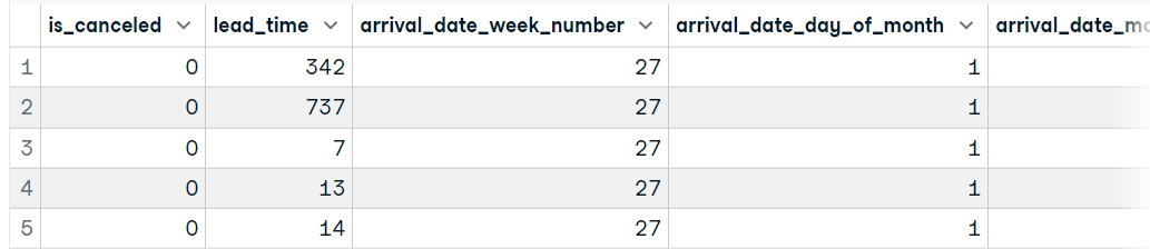
Similar to read_csv() you can also use the read.table() function to load the file. Make sure you are adding a delimiter like a comma, and header = 1. It will set the first row as column names instead of V1, V2, ...
data2 <- read.table('data/hotel_bookings_clean.csv', sep=",", header = 1)
head(data2, 5)
Importing a TXT file in R
In this part, we will use the Drake Lyrics dataset to load a text file. The file consists of Lyrics from the singer Drake. We can use the readLines() function to load the simple file, but we have to perform additional tasks to convert it into a dataframe.

Image by Author | Text file
We will use read.table’s alternative function, read.delim() to load the text file as an R dataframe. Other read.table’s alternative functions are read.csv, read.csv2, and read.delim2.
Note: by default, it is separating the values on Tab (sep = "\t")
The text file consists of lyrics and doesn't have a header row. To display all of the lyrics in a row, we need to set header = F.
You can also use other parameters to customize your dataframe, for example, the fill parameter, which sets the blank field to be added to rows of unequal length.
Read the documentation to learn about every parameter in the read.table’s alternative functions.
data3 <- read.delim('data/drake_lyrics.txt',header = F)
head(data3, 5)
Importing data from Excel into R
In this section, we will be using the Tesla Deaths dataset from Kaggle to import from Excel into R. The dataset is about tragic Tesla vehicle accidents that have resulted in the death of a driver, occupant, cyclist, or pedestrian.
The dataset contains a CSV file, and we will use MS Excel to convert it into an Excel file, as shown below.
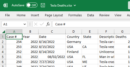
Image by Author
We will use the readxl package’s read_excel() function to read a single sheet from an Excel file. The package comes with tidyverse, but it is not the core part of it, so we need to load the package before using the function.
The function requires the location of the data and the sheet number. We can also modify how our dataframe looks by reading the description of other parameters in read_excel documentation.
library(readxl)
data4 <- read_excel("data/Tesla Deaths.xlsx", sheet = 1)
head(data4, 5)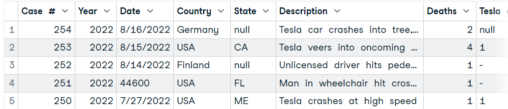
Importing data from a JSON file
In this part, we will load JSON into R using a file from the Drake Lyrics dataset. It contains lyrics, song title, album title, URL, and view count of Drake songs.

Image by Author
To load a JSON file, we will load the rjson package and use fromJSON() to parse the JSON file.
library(rjson)
JsonData <- fromJSON(file = 'data/drake_data.json')
print(JsonData[1])Output:
[[1]]
[[1]]$album
[1] "Certified Lover Boy"

[[1]]$lyrics_title
[1] "Certified Lover Boy* Lyrics"

[[1]]$lyrics_url
[1] "https://genius.com/Drake-certified-lover-boy-lyrics"

[[1]]$lyrics
[1] "Lyrics from CLB Merch\n\n[Verse]\nPut my feelings on ice\nAlways been a gem\nCertified lover boy, somehow still heartless\nHeart is only gettin' colder"

[[1]]$track_views
[1] "8.7K"
To convert the JSON data into an R dataframe,we will use the base R as.data.frame() function.
data5 = as.data.frame(JsonData[1])
data5
Importing data from a Database using SQL in R
In this part, we are going to use the Mental Health in the Tech Industry dataset from Kaggle to load SQLite databases using R. To extract the data from databases using SQL queries, we will use the DBI package and SQLite function and create the connection. You can also use similar syntax to load data from other SQL servers.
We will load the RSQLite package and load the database using the dbConnect function.
Note: You can use dbConnect to load data from MySQL, PostgreSQL, and other popular SQL servers.
After loading the database, we will display the names of the tables.
library(RSQLite)

conn <- dbConnect(RSQLite::SQLite(), "data/mental_health.sqlite")
dbListTables(conn) # 'Answer''Question''Survey'
To run a query and display the results,we will use the dbGetQuery() function. Just add a SQLite connection object and SQL query as a string.
dbGetQuery(conn, "SELECT * FROM Survey")
Using SQL within R provides you with greater control of data ingestion and analysis.
(data6 = dbGetQuery(conn, "SELECT * FROM Question LIMIT 3"))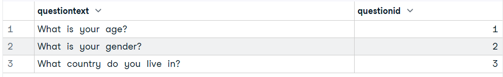
Learn more about running SQL queries in R by following the How to Execute SQL Queries in Python and R tutorial. It will teach you how to load databases and use SQL with dplyr and ggplot.
Importing data from XML and HTML files
Next, let's take a look at how to import data from two of the most popular markup languages, XML and HTML.
Importing XML into R
In this section, we will load plant_catalog XML data from w3schools using xml2 package.
Note: You can also use the XMLpackage’s xmlTreeParse() function to load the data.
Just like the read_csv() function, we can load the XML data by providing a URL link to the XML site. It will load the page and parse XML data.
library(xml2)

plant_xml <- read_xml('https://www.w3schools.com/xml/plant_catalog.xml')
plant_xml_parse <- xmlParse(plant_xml)
Later, you can convert XML data to an R data frame using the xmlToDataFrame() function.
1. Extract node set from XML data.
-
The first argument is a doc that is the object of the class
XMLInternalDocument. -
The second argument is a path, which is a string giving the XPath expression to evaluate.
2. Add the plant_node to the xmlToDataFrame() function and display the first five rows of the R dataframe.
plant_nodes= getNodeSet(plant_xml_parse, "//PLANT")

data9 <- xmlToDataFrame(nodes=plant_nodes)
head(data9,5)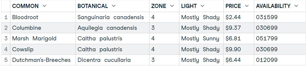
Importing HTML Table into R
This section is fun as we will be scraping the Wikipedia page of the Argentina national football team to extract the HTML table and convert it into a data frame with few lines of code.

Image from Wikipedia
To load an HTML table, we will use XML and RCurl packages. We will provide the Wikipedia URL to the getURL() function and then add the object to the readHTMLTable() function, as shown below.
The function will extract all of the HTML tables from the website, and we just have to explore them individually to select the one we want.
library(XML)
library(RCurl)

url <- getURL("https://en.wikipedia.org/wiki/Brazil_national_football_team")
tables <- readHTMLTable(url)
data7 <- tables[31]

data7$`NULL`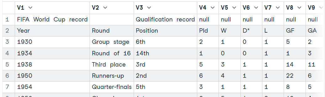
Moreover, you can use the rvest package to read HTML using URL, extract all tables, and display it as a dataframe.
-
read_html(URL)for extracting HTML data from websites. -
html_nodes(file, "table")for extracting tables from HTML data. -
html_table(tables[25])for converting HTML tables to a dataframe.
library(rvest)

url <- "https://en.wikipedia.org/wiki/Argentina_national_football_team"
file <- read_html(url)
tables <- html_nodes(file, "table")
data8 <- html_table(tables[25])

View(data8)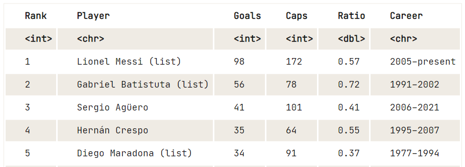
If you are facing issues while following the tutorial, you can always check out the DataLab workbook with all the code for this tutorial. Just make a copy and start practicing.
Importing Data in R From Other Data Types
The other, less popular but essential, data types are from statistical software, Matlab, and binary data.
Importing data from a SAS file
In this section, we will use the haven package to import SAS files. You can download the data from the GeeksforGeeks blog. The haven package allows you to load SAS, SPSS, and Stata files into R with minimal code.
Provide the file directory to the read_sas() function to load the .sas7bdat file as a dataframe. Read the function’s documentation to learn more about it.
library(haven)

data10 <- read_sas('data/lond_small.sas7bdat')

# display data
head(data10,5)
Importing data from a SPSS file
As we already know, we can also use the haven package to load SPSS files into R. You can download the data from the GeeksforGeeks blog and use the read_sav() function just to load the SPSS sav file.
It requires the file directory as a string and you can modify your dataframe by using additional arguments such as encoding, col_select, and compress.
library(haven)

data11 <- read_sav("data/airline_passengers.sav")
head(data11,5)
You can also use a foreign package to load a .sav file as a dataframe using the read.spss() function. The function requires only two arguments file and to.data.frame. Learn more about other arguments by reading the function's documentation.
Note: foreign package also allows you to load Minitab, S, SAS, SPSS, Stata, Systat, Weka, and Octave file formats.
library("foreign")

data12 <- read.spss("data/airline_passengers.sav", to.data.frame = TRUE)
head(data12,5)
Importing Stata files into R
In this part, we will use the foreign package to load the Stata file from ucla.edu.
The read.dta function reads Stata binary files from versions 5 through 12 and converts them into an R data frame.
Note: For Stata files from version 13 onward, use haven::read_dta() instead. The haven package supports all Stata versions and returns a tibble.
library("foreign")

data13 <- read.dta("data/friendly.dta")
head(data13,5)
Importing Matlab files into R
MATLAB is quite famous among students and researchers. The R.matlab package allows us to load the .mat file, so that we can perform data analysis and run simulations in R.
Download the MATLAB files from Kaggle to try it on your own.
library(R.matlab)

data14 <- readMat("data/cross_dsads.mat")
head(data14$data.dsads)
Importing binary files into R
In this part, we will first create a binary file and then read the file using the readBin() function.
Note: the code example is a modified version of the Working with Binary Files in R Programming blog.
First, we need to create a dataframe with four columns and four rows.
df = data.frame(
  "ID" = c(1, 2, 3, 4),
  "Name" = c("Abid", "Matt", "Sara", "Dean"),
  "Age" = c(34, 25, 27, 50),
  "Pin" = c(234512, 765345, 345678, 098567)
)
After that, create a connection object using a file() function.
con = file("data/binary_data.dat", "wb")Write the column names into the file using the writeBin() function.
writeBin(colnames(df), con)Write the value of each column into the file.
writeBin(c(df$ID, df$Name, df$Age, df$Pin), con)Close the connection after writing the data into the file.
close(con)To read the binary file, we have to create a connection to the file and use the readBin() function to display data as an integer.
Arguments used in the function:
-
conn: a connection object. -
what: an object whose mode will give the mode of the vector to be read. -
n: The number of records to be read.
con = file("data/binary_data.dat", "rb")
data15_1 = readBin(con, integer(), n = 25)

print(data15_1)Output:
[1] 1308640329    6647137    6645569    7235920    3276849    3407923
[7] 1684628033 1952533760 1632829556 1140875634    7233893  838874163
[13]  926023733    3159296  892613426  922759729  875771190  875757621
[19]  943142453  892877056
You can also convert the data from binary to a string by replacing integer() with character() in the what argument.
Read the readBin() function documentation to learn more.
con = file("data/binary_data.dat", "rb")
data15_2 = readBin(con, character(), n = 25)

print(data15_2)Output:
[1] "ID"     "Name"   "Age"    "Pin"    "1"      "2"      "3"      "4"
[9] "Abid"   "Matt"   "Sara"   "Dean"   "34"     "25"     "27"     "50"
[17] "234512" "765345" "345678" "98567"
Learn how to import flat files, statistical software, databases, or data right from the web by taking our Intermediate Importing Data in R course.
Importing Data into R using QuantMod
Quantmod is a financial modeling and trading framework for R. We will be using it to download and load the latest trading data in the form of a dataframe.
We will use quantmod’s getSymbols() function to load Google stock's historical data by providing “from” and “to” dates and “frequency”. Learn more about the quantmod package by reading the documentation.
library(quantmod)

getSymbols("GOOGL",
          from = "2022/12/1",
          to = "2023/1/15",
          periodicity = "daily")
# 'GOOGL'
The data is loaded in a GOOGL object, and we can view the first five rows by using the head() function.
head(GOOGL,5)Output:
GOOGL.Open GOOGL.High GOOGL.Low GOOGL.Close GOOGL.Volume
2022-12-01     101.02     102.25    100.25      100.99     28687100
2022-12-02      99.05     100.77     98.90      100.44     21480700
2022-12-05      99.40     101.38     99.00       99.48     24405100
2022-12-06      99.30      99.78     96.42       96.98     24910700
2022-12-07      96.41      96.88     94.72       94.94     31045400
          GOOGL.Adjusted
2022-12-01         100.99
2022-12-02         100.44
2022-12-05          99.48
2022-12-06          96.98
2022-12-07          94.94
Importing Large Datasets into R
Importing a large file is tricky. You need to make sure that the function is optimized for memory-efficient storage and fast access.
In this section, we will be looking at popular functions used for loading CSV files greater than 1 GB. We are using the US Accidents (2016 - 2021) dataset from Kaggle, which is about 1.15GB in size and has 2,845,342 records.

Import a large dataset into R using read.table()
We can load the zip file directly into utils’s read.table() function by using the unz function. It will save you time to extract and then load the CSV file.
-
Provide
unzwith the zip directory and the CSV file within the zip. -
After that, add the
unzobject to theread.table()function. -
To load data faster, we will be limiting the
nrowsto 10,000. -
By default, it separates the values on space, so make sure you are providing a
separgument with a comma.
file <- unz("data/US Accidents.zip", "US_Accidents_Dec21_updated.csv")

(data16 <- read.table(file, header=T, sep=",",nrow=10000))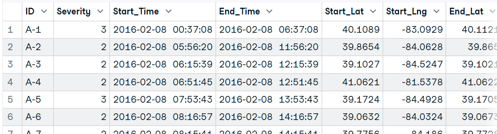
Import a large dataset into R using read.csv()
Similar to read.table(), we can use readr’s read_csv() function to load the CSV file. Instead of nrow, we will use n_max to read a limited number of records.
In our case, we are not restricting any data and allowing the function to load full data.
Note: it almost took a minute to load the full data. You can change the number of threads to reduce loading time. Learn more by reading the function documentation.
(data17 <- read_csv('data/US_Accidents_Dec21_updated.csv'))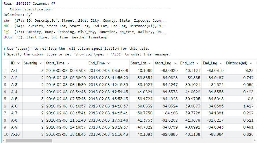
Import a large dataset using the ff package
We can also use the ff package to optimize loading time and storage. The read.table.ffdf() function loads data in chunks, reducing the loading time.
We will first unzip the file and read the data using the read.table.ffdf() function.
unzip('data/US Accidents.zip',exdir='data')

library(ff)

data18 <- read.table.ffdf(file="data/US_Accidents_Dec21_updated.csv",
                          nrows=10000,
                          header = TRUE,
                          sep = ',')
data18[1:5,1:25]
In the end, we will look at the most commonly used function fread() from the data.table package to read the first 10,000 rows. The function can automatically understand file format, but in rare cases, you have to provide a sep argument.
For a deeper dive into data.table syntax and operations, check out our data.table R Tutorial.
library(data.table)

(data19 <- fread("data/US_Accidents_Dec21_updated.csv",
              sep=',',
              nrows = 10000,
              na.strings = c("NA","N/A",""),
              stringsAsFactors=FALSE
              ))
Importing Parquet files with Arrow
Parquet is a columnar storage format increasingly used for large analytical datasets. The arrow package reads Parquet files into R with high performance and low memory usage.
library(arrow)

parquet_data <- read_parquet("data/example.parquet")
head(parquet_data, 5)
Arrow also supports reading from S3 buckets and Google Cloud Storage. For datasets too large to fit in memory, use open_dataset() to process files in chunks without loading everything at once.
Dataset Reference
If you want to try the code examples on your own, here is the list of all of the datasets used in the tutorial.
- CSV: Hotel Booking Demand
- TXT: Drake Lyrics
- Excel: Tesla Deaths
- JSON: Drake Lyrics
- SQL DB: Mental Health in the Tech Industry
- XML: w3schools
- HTML: Argentina national football team
- SAS: SAS Files - GeeksforGeeks
- SPSS: SPSS Files - GeeksforGeeks
- Stata: Applied Regression Analysis by Fox Data Files
- Matlab: Cross-position activity recognition | Kaggle
- Large Dataset: US Accidents (2016 - 2021)
Final Thoughts
R handles a wide range of data formats out of the box, from CSV and Excel to SQL databases and statistical software files. Once your data is loaded, you can move into cleaning with the Cleaning Data in R course, then into exploratory analysis and visualization.
In this tutorial, we have learned how to load all kinds of datasets using the popular R packages for better storage and performance. If you want to start your data science career with R, check out our Data Scientist with R career track. It consists of 24 interactive courses that will teach you everything about R programming, statistical analysis, data handling, and predictive analysis. You can also take a certification exam after completing the track.
Also, check out the Import Data Into R DataLab workbook, which comes with source code, outputs, and a data repository. You can make a copy and start learning on your own.