Analyzing Credit Card Transactions using R

Credit card transaction analysis is a important process for financial institutions and businesses to detect fraud, understand customer spending habits and enhance security. Using R Programming Language , we can effectively perform data analysis, visualize spending patterns and create predictive models for fraud detection.

Project Overview

In this project, we aim to analyze a credit card transaction dataset to detect fraudulent activities using R. We will go through the following steps:

1. Load libraries and the dataset.
2. Preprocess the data to handle missing values, normalize numerical features and split the dataset into training and testing sets.
3. Perform Exploratory Data Analysis (EDA) to visualize trends, correlations and patterns in the dataset.
4. Build a logistic regression model for fraud detection.
5. Evaluate the model using accuracy, precision, recall and F1 score.

By the end of this analysis, we will gain insights into customer transaction patterns and develop a model to predict fraudulent activities.

Dataset Overview

A credit card transactions dataset typically includes the following columns:

1. Time: The number of seconds elapsed between this transaction and the first transaction in the dataset. This helps in understanding the time pattern of transactions.
2. Amount: The transaction amount. This is crucial for detecting large transactions or anomalies.
3. Class: This is often a binary variable indicating whether the transaction is fraudulent (1) or not (0).
4. V1, V2, ..., V28: Principal components obtained using PCA (Principal Component Analysis) to anonymize the data.

Dataset Link: Credit Card Transactions

1. Loading the required Libraries and Dataset

We will begin by loading the necessary libraries and importing the dataset.

library(tidyverse)
library(caret)
library(corrplot)

data <- read.csv("/content/creditcard.csv")

head(data)

Output:

2. Data Preprocessing

We will handle missing values, scale the Amount column to standardize it and split the dataset into training (70%) and testing (30%) sets.

sum(is.na(data))

data$Amount <- scale(data$Amount)

set.seed(123)
train_indices <- sample(1:nrow(data), 0.7 * nrow(data))
train_data <- data[train_indices, ]
test_data <- data[-train_indices, ]

Output:

[1] 0

We ensured the data was clean by checking for missing values and scaling the Amount column. We also split the dataset into training and testing sets to evaluate the model later.

3. Exploratory Data Analysis (EDA)

We will explore the distribution of the target variable Class, perform correlation analysis and visualize trends in the data.

• We will understand the distribution of variables helps in identifying patterns.
• Examine the relationships between features can reveal insights into the data.

3.1. Distribution of the Target Variable

Now we will visualize the Distribution of the Target Variable.

ggplot(train_data, aes(x = factor(Class))) +
  geom_bar(fill = "steelblue") +
  labs(title = "Distribution of Normal and Fraudulent Transactions",
       x = "Class",
       y = "Count")

Output:

The Class distribution showed an imbalance, with more non-fraudulent transactions.

3.2. Correlation Analysis

Now we will calculate and visualize Correlation Analysis.

cor_matrix <- cor(train_data[, -1])
corrplot(cor_matrix, method = "circle", type = "upper")

Output:

The correlation matrix depicts the relationships between PCA components.

3.3. Visualization of Spending Trends

We will visualize how spending changes over time by creating line graphs.

data$Time_hours <- data$Time / 3600

ggplot(data, aes(x = Time_hours, y = Amount)) +
  geom_line(color = "blue") +
  labs(title = "Spending Trends Over Time",
       x = "Time (hours)",
       y = "Normalized Amount")

Output:

The normalised amount provides insights into transaction patterns.

3.4. Visualizing Transaction Volumes

We can use histograms to visualize the distribution of transaction amounts.

ggplot(data, aes(x = Amount)) +
  geom_histogram(binwidth = 0.1, fill = "steelblue", color = "black") +
  labs(title = "Distribution of Transaction Amounts",
       x = "Normalized Amount",
       y = "Frequency")

Output:

The normalized amount v frequency provides insights into transaction pattern's frequency.

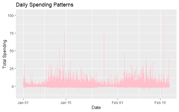
3.5. Daily Spending Patterns

We will convert the Time_hours to a date format and summarize spending by date.

data$Date <- as.Date(data$Time_hours, origin = "1970-01-01")

daily_spending <- data %>%
  group_by(Date) %>%
  summarise(Total_Spending = sum(Amount))

ggplot(daily_spending, aes(x = Date, y = Total_Spending)) +
  geom_line(color = "pink") +
  labs(title = "Daily Spending Patterns",
       x = "Date",
       y = "Total Spending")

Output:

4. Building the Model

Now we will build a logistic regression model using the training data to predict fraudulent transactions.

model <- glm(Class ~ ., data = train_data, family = binomial)

summary(model)

Output:

The analysis identified significant predictors such as V1, V4, V8 and V10 that are likely linked to fraudulent transactions.

5. Evaluating the Model

We will evaluate the model's performance using the test data and calculate key metrics like accuracy, precision, recall and F1 score.

pred_prob <- predict(model, test_data, type = "response")
pred_class <- ifelse(pred_prob > 0.5, 1, 0)

confusionMatrix <- table(Predicted = pred_class, Actual = test_data$Class)
print(confusionMatrix)
cat("---------------","\n")

accuracy <- sum(diag(confusionMatrix)) / sum(confusionMatrix)
precision <- confusionMatrix[2, 2] / sum(confusionMatrix[2, ])
recall <- confusionMatrix[2, 2] / sum(confusionMatrix[, 2])
f1_score <- 2 * (precision * recall) / (precision + recall)

cat("Accuracy: ", accuracy, "\n")
cat("Precision: ", precision, "\n")
cat("Recall: ", recall, "\n")
cat("F1 Score: ", f1_score, "\n")

Output:

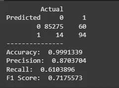
The model achieved an accuracy of 99.91%, a precision of 87.04%, a recall of 61.04% and an F1 score of 71.76%. This indicates that the model is effective in predicting fraudulent transactions, though there is room for improvement in recall.

Conclusion

From our analysis, we:

• Explored the distribution of normal vs. fraudulent transactions and identified data imbalances.
• Performed correlation analysis and visualized spending trends over time.
• Built a logistic regression model that performed well in detecting fraudulent transactions.

We concluded that the logistic regression model is an effective tool for fraud detection in credit card transactions. Further improvements can be made by optimizing the model and balancing the dataset for better recall.