HLOOKUP is used to search for a value in the top row of a table and return data from a specified row below. It is ideal for horizontally organized data and complements VLOOKUP, which is used for vertical lookups.
- Searches for a value in the first row of a table.
- Returns the corresponding value from a specified row in the same column.
Applications
The HLOOKUP function is most useful when:
- Data is arranged horizontally in rows.
- You need to fetch values from a specific row using a lookup value in the top row.
- You are working with exact or approximate matches in structured datasets.
Syntax and Parameters
The syntax of the HLOOKUP function is as follows:
HLOOKUP(lookup_value, table_array, row_index_num, [range_lookup])
Where:
- lookup_value: The value we want to search for in the top row of the table.
- table_array: The range of cells that contains the data. The top row of this range will be searched for the lookup_value.
- row_index_num: The row number in the table_array from which to return a value. The top row is row 1.
- [range_lookup]: An optional argument. Use TRUE for an approximate match (default), or FALSE for an exact match.
Steps to Use HLOOKUP
The HLOOKUP formula is a useful tool for looking up data in tables arranged horizontally. This HLOOKUP tutorial will guide you through the steps to use the function effectively:
Step 1: Preparing our Data
We organize our data so that the lookup value resides in the first row of a range or table.
Example:

Step 2: Choose a Cell to Enter the Formula
Select a blank cell where we want the result of the HLOOKUP function to appear. In the below example we have selected B5.

Step 3: Enter the HLOOKUP Formula
To look up the sales for Q3, enter the following formula in your selected cell:
Syntax:
=HLOOKUP("Q3", A1:E2, 2, FALSE)
Step 4: Press Enter
After pressing Enter, Excel will return 2500, which is the value in the second row under "Q3."

Excel HLOOKUP Function
The HLOOKUP function is an efficient tool in Excel that helps us find data arranged horizontally in a table. In this section, we’ll explore HLOOKUP examples in Excel that demonstrate how to use the function for quick and efficient data retrieval.
Example 1: Finding an Exact Match
Suppose we have a grade table where the first row contains scores and the second row contains grades.

To find the grade for a score of 80, use the formula:
=HLOOKUP(80, A1:F2, 2, FALSE)
Result: Excel will return B.

Example 2: Approximate Match in HLOOKUP
For approximate matches, set the range_lookup argument to TRUE.
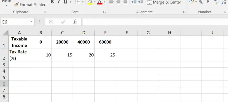
To find the tax rate for an income of 45000, use the formula:
=HLOOKUP(45000, A1:E2, 2, TRUE)
Result: Excel will return 20, as 45000 is between 40000 and 60000.
Approximate match works only when the top row is sorted in ascending order.
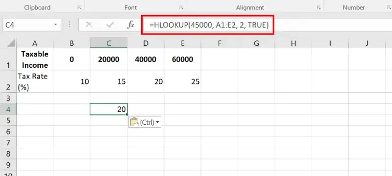
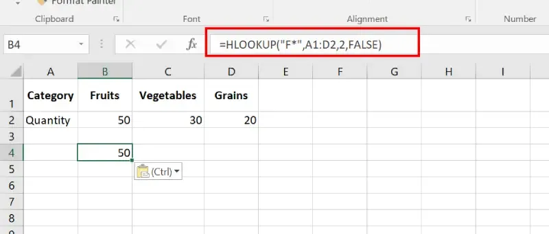
Example 3: Using Wildcards with HLOOKUP
Using Asterisk (*) for Partial Matches. we want to find a value in the top row that matches a pattern starting with ‘F'.

Formula:
=HLOOKUP("F*",A1:D2,2,FALSE)
Result: 50 (The quantity for "Fruits").
Steps to Use HLOOKUP Across Two Worksheet
Using the HLOOKUP formula across two worksheets in Excel is a great way to retrieve data from one sheet while working on another. This can be especially helpful when managing large datasets spread over multiple sheets.
Let's Suppose we have two worksheets: Sheet1 and Sheet2. To extract our matching data from another worksheet, mention the sheet name followed by an exclamation mark.
Step 1: Identify the Lookup Value
In Sheet1, locate the cell containing the lookup value (e.g., B1) that we want to search for in Sheet2.

Step 2: Specify the Data Range in the Other Sheet
We define the data range from the second sheet to power our HLOOKUP. This step ensures our formula targets the correct table across sheets. Let’s set it accurately.
- We reference Sheet2 in our formula by including the sheet name followed by an exclamation mark (!).
- We use an example data range in Sheet2: A1:F2.
- We confirm the range covers the top row and the data row we need.
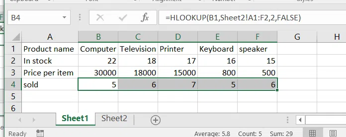
Step 3: Write the HLOOKUP Formula
Enter the HLOOKUP formula by referencing Sheet2 to fetch the required data.
- In Sheet1, input the following formula to perform the lookup
=HLOOKUP(B1, Sheet2!A1:F2, 2, FALSE)
- We note B1 as the lookup value in Sheet1.
- We confirm Sheet2!A1:F2 as the data range in Sheet2 containing the lookup table.
- We set 2 to specify the row number in the lookup table from which to retrieve the result.
- We use FALSE to ensure an exact match.
Step 4: Drag the Formula
Drag the formula down or across other cells in Sheet1 to copy the HLOOKUP formula, dynamically referencing the lookup values.
Data from sheet 2 is copied from sheet 2 to sheet 1.
Steps to Use HLOOKUP with Another Workbook
The HLOOKUP function in Excel becomes even more efficient when we use it to retrieve data across multiple workbooks. This can help you manage large datasets stored in different files without the need to combine them manually.
Suppose we have two workbooks: Workbook1.xlsx and Workbook2.xlsx. we want to retrieve data from Workbook2.xlsx into Workbook1.xlsx.
Step 1: Open Both Workbooks
Ensure both workbooks are open in Excel.
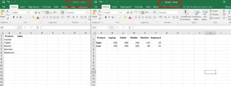
Step 2: Reference the External Workbook
In Workbook1.xlsx, write the formula referencing Workbook2.xlsx. The external workbook name should be enclosed in square brackets ([]) and followed by the sheet name and range.
Step 3: Write the HLOOKUP Formula in Book1.
For example, to retrieve data from Sheet1 of Workbook2.xlsx, use the following formula:
=HLOOKUP(A2, [Workbook2.xlsx]Sheet1!A1:F2, 2, FALSE)

Step 4: Save the Formula
If the external workbook is closed, the file path will be automatically included in the formula.
Example:
=HLOOKUP(A2, 'C:\Documents\[Workbook2.xlsx]Sheet1'!A1:F2, 2, FALSE)
Step 5: Copy the Formula
Copy or drag the formula to other cells as needed to reference corresponding lookup values.

This setup shows how HLOOKUP works between two workbooks, retrieving data dynamically from the Sales row in Workbook2.xlsx into Workbook1.xlsx.
Key Points for HLOOKUP Function
- The lookup value must be in the top row of the table array.
- The table array should contain multiple rows and columns.
- HLOOKUP is not case-sensitive (e.g., “jane” = “Jane”).
- If no match is found, it returns #N/A.
- For approximate matches, the top row must be sorted in ascending order.
VLOOKUP vs. HLOOKUP
VLOOKUP and HLOOKUP are both lookup functions in Excel, but they work differently based on how the data is organized.
| Feature | VLOOKUP | HLOOKUP |
|---|---|---|
| Orientation | Searches data vertically (columns) | Searches data horizontally (rows) |
| Search Direction | Looks in first column and returns value from a specified column in the same row | Looks in first row and returns value from a specified row in the same column |
| Best Use | When data is arranged in columns | When data is arranged in rows |