Pivot Table Slicers in Excel

Pivot Table Slicers make data filtering in Excel simple, fast, and interactive. They replace drop-down filters with easy visual buttons, improving dashboards and enabling quick multi-filtering across pivot tables. Overall, slicers make data analysis more efficient and user-friendly.

Inserting a Pivot Table Slicer

Follow the steps below to insert a Pivot table slicer:

• Step 1: Create a Pivot Table: Select the data we want to analyze and then create a Pivot table.
• Step 2: Design the Pivot Table: Design the Pivot table by dragging the relevant fields to the Rows, Columns, Values or Filters area of the PivotTable Fields pane.
• Step 3: Insert a Slicer: When our Pivot Table is ready, go to the Pivot Table Analyze or Options tab in the Excel ribbon. Click on Insert Slicer and a dialog box will appear, with all the fields available in the Pivot Table.

• Step 4: Choose a Field for the Slicer: Select the field we want to use as a slicer and click OK.

Working with Slicers

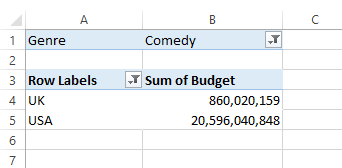
Let’s understand slicers with an example using an IMDb dataset of 2016 movies, including ratings, budget, revenue, country, and genre. Suppose we want the total budget by country filtered by genre, such as comedy movies in the U.S.A and U.K.

We can filter this data in two ways:

1. Using the Pivot Table filter: Drag the Genre field into the filter box in the Pivot Table field list and select the desired genres.

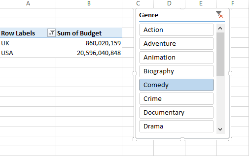
2. Using a slicer: Insert a slicer for the Genre field and select the required genres using visual buttons.

Note: Both Pivot Table filters and slicers return the same results, but slicers provide a more interactive and user-friendly way to filter data.

To select multiple items in a slicer, use the Multi-select option or hold the Ctrl key while selecting multiple genres. For example, selecting both Comedy and Crime will show combined results for those genres.

Formatting Slicers

When you insert a slicer, a new Slicer Tools menu appears in the ribbon which offers various options to customize our slicer’s appearance.

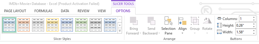
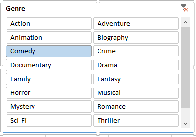
1. If our slicer contains many items, we can increase the number of columns to make it wider and display the items more neatly.

2. Additional formatting options are available under Slicer Settings where we can:

• Choose to show or hide the slicer header.
• Sort the slicer items in ascending or descending order.
• Adjust other display preferences to suit our needs.

Steps to Adjust Slicers in Excel

After inserting slicers we may want to move, resize or customize them to fit our worksheet and improve usability. Excel provides several options to help us do this easily.

1. Moving a Slicers

To move a Slicer to a new location on the same worksheet, follow these steps:

• Point to the Slicer's border or any empty part of the Slicer.
• When the pointer changes to a 4-headed arrow, drag the slicers to their new position.

2. Resizing a Slicer

Follow the steps to resize a Slicer to make it larger or smaller:

• Click on the slicer to select it.
• Point to one of the sizing handles on its border.
• When the cursor changes to a two-headed arrow, drag inward or outward to adjust the size.

3. Change Slicer Style

Excel has some built-in styles similar to Pivot Tables. To change the style:

• Click on an empty part of the Slicer to select it.
• On the Excel Ribbon, go to the Slicer tab.
• In the Slicer Styles group, click on one of the visible styles to apply it to the Slicer.

4. Change Slicer Settings

We can modify various slicer settings to control its appearance and behavior:

1. Sort Order:

• Step 1: Right-click on the Slicer and click Slicer Settings.
• Step 2: In the Item Sorting and Filtering section, select Ascending or Descending as per our preference.
• Step 3: Click OK to apply changes.

2. Change Slicer Captions:

• Step 1: Right-click on the Slicer and Click Slicer Settings.
• Step 2: In the Header Section, type the desired caption text to replace the existing caption.
• Step 3: Click ok to save the changes.

5. Multiple Slicers

• Multiple slicers can be used to filter data based on more than one column. For example, Genre and Language slicers together can filter Hindi Comedy movies in the USA and UK.

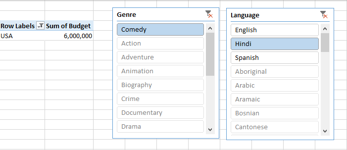
So from the picture above, we can see that there are no Hindi comedy films in the U.K.

Linking a Slicer to Multiple Pivot Tables

We can link our slicer to multiple pivot tables which can build a very interactive dashboard. To do so follow the below steps:

Step 1: Right-click on the slicer and select the option of Report Connections.

Step 2: After that, we will see a menu like this.

Step 3: Now select all the table names on which we want our slicer to work.

For example, using the IMDb movies dataset we might want the slicer to filter both the budget and gross revenue pivot tables simultaneously for all comedy films in the U.S.A and U.K. Linking the slicer helps it to update both tables at once.

So here our slicer works on both the pivot tables.