Sorting Pivot Tables in Excel helps organize large datasets in a meaningful way, making it easier to identify trends, compare values, and draw insights quickly. You can sort data by labels, values, or custom order to improve clarity and analysis. These sorting options are useful for tasks like sales reporting, budgeting, and data comparison.
Benefits of Sorting in Pivot Tables
- Data Clarity: Organizes labels or values for easier interpretation.
- Focused Analysis: Highlights key metrics (e.g., highest sales).
- Custom Reporting: Tailors data order for specific needs (e.g., custom sequences).
- Efficient Navigation: Simplifies large datasets by prioritizing relevant information.
Types of Pivot Table Sorting
- Label Sorting: Sort row or column labels alphabetically or in reverse alphabetical order.
- Value Sorting: Sort data based on numerical values, such as totals or averages, in ascending or descending order.
- Custom Sorting: Arrange data in a specific order, such as months, days of the week, or a custom-defined sequence.
Sort a Pivot Table in Excel
Follow the steps below to sort data in a Pivot Table:
Method 1: Sorting by Labels
Step 1: Open the Excel sheet that contains the Pivot Table.

Step 2: Click on the drop-down arrow next to the Row Labels or Column Labels heading in the Pivot Table.
Step 3: Select Sort A to Z for ascending order or Sort Z to A for descending order.

Method 2: Sorting by Values
Step 1: Select any cell containing a value in the Pivot Table.
Step 2: Right-click on the selected cell.
Step 3: Click on Sort and choose:
- Smallest to Largest for ascending order
- Largest to Smallest for descending order

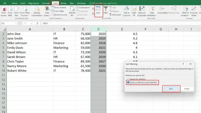
Custom Sorting
Step 1: Select any cell in the Pivot Table.
Step 2: Go to the Data tab in the ribbon.
Step 3: Click on the Sort option.
Step 4: In the Sort dialog box, choose the field you want to sort.
Step 5: Under the Order section, select Custom List.

Step 6: Choose or create a custom sequence (e.g., months or weekdays).

Step 7: Click OK to apply the custom sorting.
