Add Filters in MS Excel

Excel filters allow us to focus on specific data in large datasets, such as equipment types or demographics, by hiding irrelevant rows.

Applying Filters in Excel

Filters help us isolate data, like laptops and projectors in an equipment log. Follow these steps:

Step 1: Preparing our Data

Make sure our worksheet has a header row that names each column. This is important for filters to work properly.

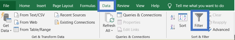
Step 2: Enable Filters

Select the Data tab and then click the Filter command.

Step 3: Apply a Filter

Drop-down arrows will appear next to each header. Click the drop-down arrow for the column we want to filter. For example, to filter equipment types, click the arrow in column C.

Step 4: Deselect All Data

The Filter menu will appear. Uncheck the box next to Select All to quickly deselect all data.  

Step 5: Select Required Data

Check the boxes next to the data we want to filter and then click OK. In this example, we will check Laptop and Tablet to view only those types of equipment. 

Step 6: View Filtered Results

The worksheet will now display only the selected equipment and temporarily hide all other rows.

Filtering options can also be accessed from the "Sort & Filter" command on the Home tab.  

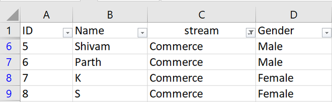
Applying Multiple Filters

Filters in Excel work together so we can apply more than one filter to narrow down our data. For example, if we've already filtered the worksheet to show only the humanities stream we can add another filter to display only records where the gender is Female.

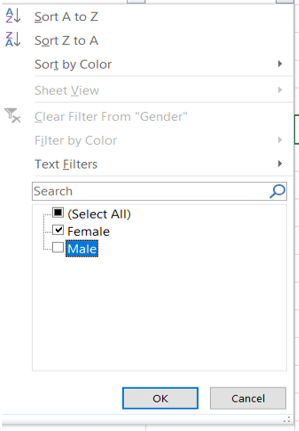
Step 1: Select the Next Column

Click the drop-down arrow for the column we want to filter next. In this case, column D for Gender.

Step 2: Open the Filter Menu

The Filter menu will appear.

Step 3: Choose Filter Criteria

Select or deselect the options as needed. For example, uncheck all except Female then click OK.

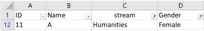
Step 4: View Filtered Results

The new filter will be applied. In our example, the worksheet is now filtered to show only female students in the Humanities stream.

Clearing Filters

After applying a filter, we may want to remove or clear it from our worksheet, so we'll be able to filter content in different ways.

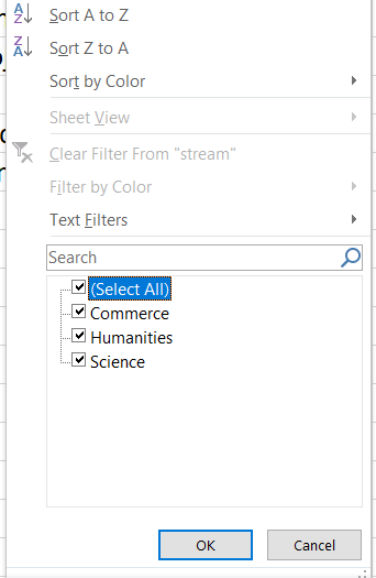
Step 1:Select the Filtered Column

Click the drop-down arrow for the column with the filter we want to clear. For example to clear the filter in column D, click the arrow in column D.

Step 2: Open the Filter Menu

The Filter menu will appear.

Step 3: Clear the Filter

Choose Clear Filter from [COLUMN NAME] from the Filter menu. In our example, we'll select Clear Filter from "Stream".  

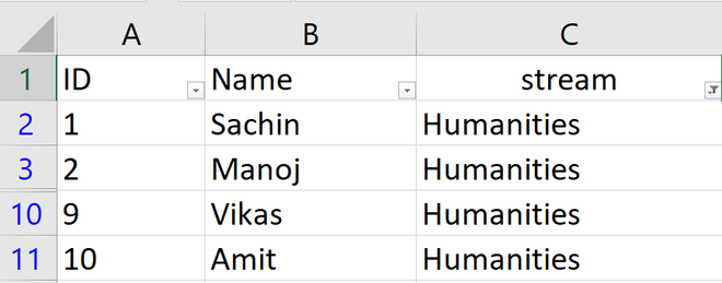
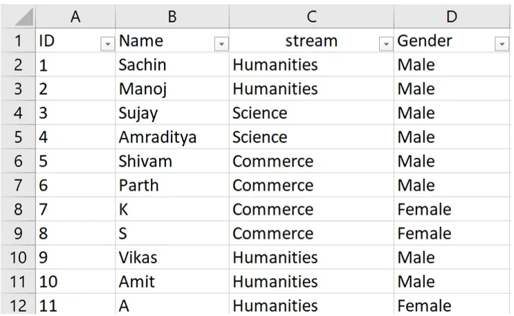
Step 4: View Updated Data

The filter will be cleared from the column. The previously hidden data will be displayed. The data displayed is given below:

Filters turn a messy spreadsheet into something simple and manageable helps in making data work feel a bit less like work and a lot more like solving a puzzle.