Flattening data in an Excel Pivot Table is the process of converting hierarchical data into a simple table where each row contains complete information and labels are repeated. This makes the data easier to analyze, filter, and use for reporting or exporting.
Benefits of Flattening Data in Excel
- Improved Data Analysis: Flattened data is easier to analyze, as all relevant information is available in a tabular format.
- Enhanced Data Extraction: Flattened data can be more easily extracted and imported into other systems or data warehouses.
- Simplified Reporting: Creating reports becomes more straightforward with data in a flat format.
How do we use flatten in Excel
Excel has a capability called =FLATTEN(), which changes over a reach, or different reaches, into a solitary section. For example, if the following table was in A1:C3...
| 1 | 2 | 3 |
|---|---|---|
| 4 | 5 | 6 |
| 7 | 8 | 9 |
If we entered =UNIQUE(A1:C3) in A5, we would get the following dynamic range output,
| 1 |
|---|
| 2 |
| 3 |
| 4 |
| 5 |
| 6 |
| 7 |
| 8 |
| 9 |
Given this is a dynamic range output, it can then be used in things like UNIQUE, FILTER, SORT, and so on, or referred to in one more regular formula as A5#.
Steps to Flatten a Pivot Table in Excel
This technique comes from preparing Excel data for import into a data warehouse. Sometimes, data is provided in a PivotTable format, which is not ideal for analysis or extraction, especially because all row labels are placed in a single column by default.

In order to make the format more usable, it's possible to "flatten" the pivot table in Excel. To do this, click anyplace on the pivot table to activate the PivotTable Tools menu. Click Design, then Report Lawet and then Show in Tabular Form.
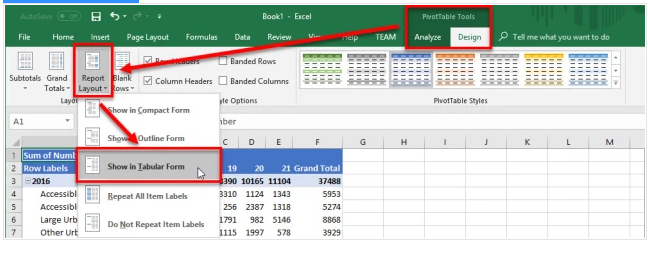
This will separate out the row labels and make it simpler to explore data.

Steps to Flatten, Repeat, and Fill Labels Down in Excel
Many Excel features, such as PivotTables, charts, AutoFilter, and Subtotal, are designed to work with structured (flat) data, where every cell in the table contains a value.
- In this format, all information about a record is stored within its row, rather than depending on its position in the table.
- This makes it easy to distinguish from non-flat data, where values may be missing or spread across rows in a less structured way.

We can see labels are not repeated, and there are cells with missing values. Hence, we should decide on data about a record in view of the place of the line inside the table.

Summary
- Select a range that we want to flatten - typically, a column of labels.
- Highlight the empty cells only - hit F5 (GoTo) and select Special > Blanks.
- Type equals (=) and then the Up Arrow to enter a formula with a direct cell reference to the first data label.
- Instead of hitting enter, hold down Control and hit Enter.
- To replace the formulas with values, select the entire column, and then Copy/Paste Special > Values
Step 1: First, select the range that we'd like to flatten. This is typically a column of labels we want to repeat, represented by B39:B62 as shown image.

Step 2: Next, we want to select only the empty cells within the range. We can simply use the Go To order for this.
Hit the F5 key on wer keyboard to bring up the Go To dialog, as shown image.

Then, hit the Special button to raise the Go To Special dialog as shown in the image.
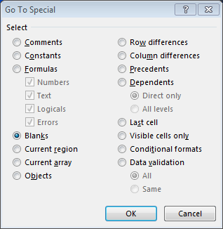
Click OK, and Excel will select only the empty/blank cells within the original range, as shown in the image.

Step 3: To pull the value from the cell above, type = and press the Up Arrow key to automatically reference the cell above. Avoid pressing Enter immediately, as the formula should first appear in the cell before confirming it.

Step 4: To fill the formula across all selected cells, hold the Ctrl key and press Enter after typing the formula. If Enter was already pressed, retype the formula and use Ctrl + Enter instead, as this shortcut both confirms the formula and fills it into all selected cells at once.

Step 5: To replace formulas with values, first select the entire section, ensuring only a single column range is selected. Copy the range, then use Paste Special and choose Values to convert all formulas into their final values.

When we click OK, we are finished. We repeat these steps on the Account column, flat data as shown in the image:

Note: You can typically perform this task on multiple columns at the same time, it only works if the first row has values for all selected columns, so, just be sure to review and doublecheck your work.