Locking formulas in Microsoft Excel helps prevent accidental changes and keeps your calculations accurate. By protecting formula cells, you can allow users to edit only specific parts of a spreadsheets while keeping important calculations safe. In this guide, you will learn simple methods to lock formulas and protect your Excel data effectively.
Understanding Cell References in Excel
Before we explore the $ shortcut, it's crucial to grasp the concept of cell references. In Excel formulas, cell references indicate which cells to include in calculations. There are three main types of cell references:
Relative References
- Default in Excel (e.g.,
A1) - Adjust automatically when formulas are copied to other cells.
Absolute References
- Stay fixed during copying (e.g.,
$A$1) - Created using the dollar (
$) sign before the column and row.
Mixed References
These references enable you to lock either the column or row, but not both. Create a mixed reference by adding a $ symbol before either the column letter or row number, such as $A1 or A$1.
How to Lock Formula in Excel with Dollar Sign
In this section, we’ll provide a step-by-step guide on how to lock formulas using the dollar sign to create absolute references. This method is vital for maintaining consistent references in your calculations.
Step 1: Open the Spreadsheet
Open the Excel sheet where your formula is written.

Step 2: Lock the Formula Reference
In this sheet we want to multiply the price with the units to calculate total units for every day.
Enter the formula for one row as shown below.

Step 3: Locking the Reference to Cell B1
Now, we want to lock the reference to the cell "B1" because we want it to stay same for all the rows. When the formula is dragged the value of "B1" cell should remain the same.
Place the cursor at the end of B1 which is entered in the formula shown in the cell "C4" in the below image.

Press "F4". You can confirm that the reference to the cell "B1" is locked when you see dollar sign($) placed in front of "B1" in the formula. As shown in the image below, like "$B$1".

Step 4: Preview Result
Press "Enter", you will see that the value is been calculated.

Step 5: Drag the formula to apply it to all the rows

How to Lock Formulas in Excel Without Protecting the Workbook
Learn how to lock formulas while keeping the workbook accessible. This method allows users to edit other cells without altering locked formulas, ensuring data integrity.
Step 1: Open the spreadsheet
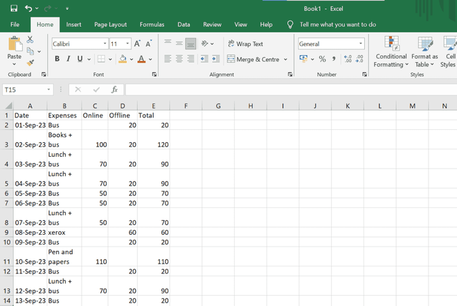
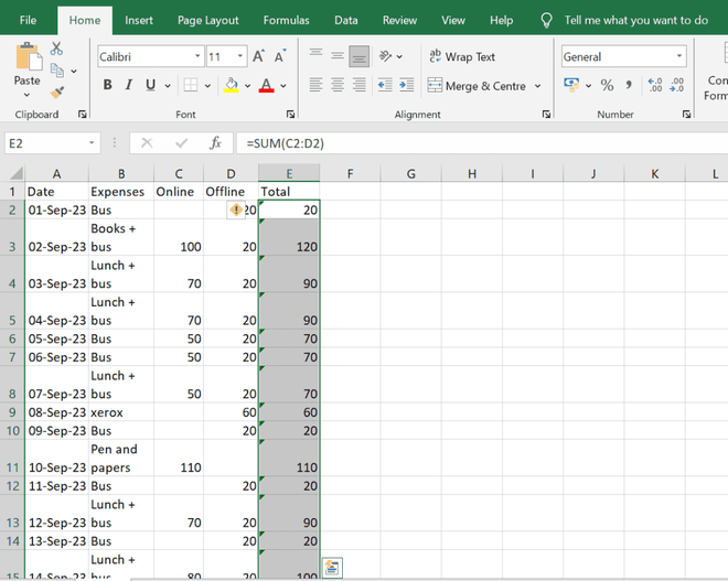
Suppose we have an Excel as follows which contains some calculations done with the help of formulas.
Step 2: Unlock all Cells
1. Select the whole excel sheet by pressing Ctrl + A.

Step 3: Right- Click and Select Format Cells
Right click while the cells are selected. Click on "Format Cells" option or Press Ctrl + 1.
-660.png)
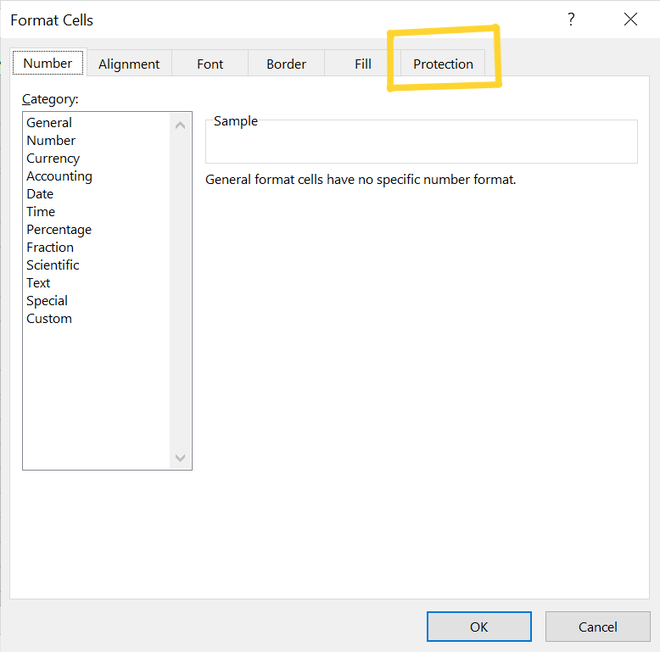
Step 4: Go to the Protection Tab
The below box will now open. Choose the "Protection" tab.
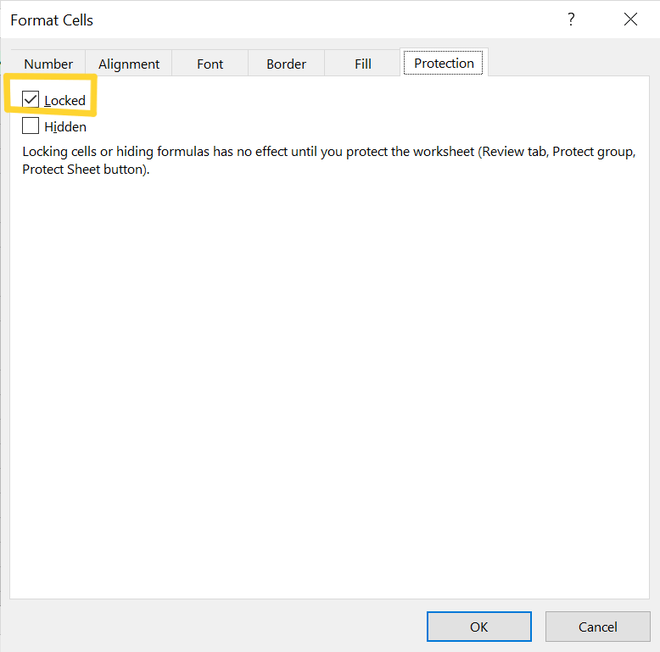
Step 5: Unmark the Locked Checkbox and Click Ok
Observe the "Locked" option is marked. Unmark this checkbox
Step 6: Select the cells with formulas
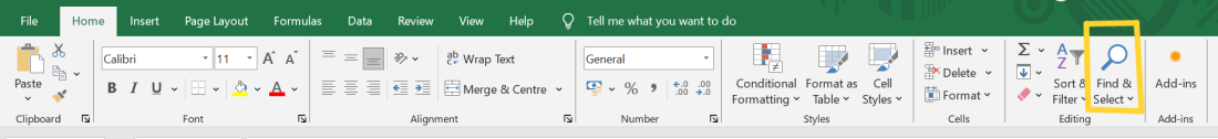
1. Next go to the "Home" section. Select "Find & Select" option.
2. Completing the above step will open a dialog box as shown below. Click on "Go to Special".

3. This will open a separate dialog box as shown below.
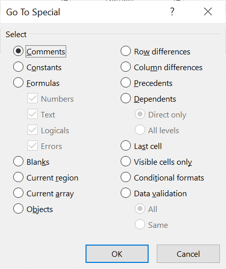
4. Choose the "Formulas" option. Click "Ok".

5. After the above step. All the cells containing formulas will be selected as shown below.
Step 7: Lock the cells
1. Now press Ctrl + 1. In the "Protection" tab check the "Locked" and "Hidden" option.

2. The options will look as below. Click "Ok". All the cells containing formulas are now locked and hidden.

Step 8: Protect the cells
1. While the all the locked formula cells are still selected. Go to "Review" section.

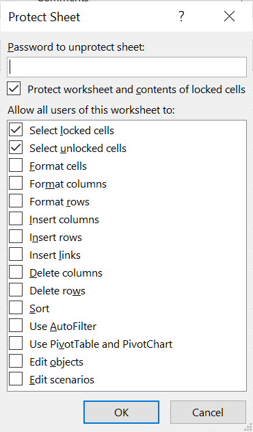
2. Choose the "Protect Sheet" option.

3. Now in the "Protect Sheet" dialog box, enter a password to secure the sheet. After you have entered the password click "Ok".
4. Confirm the password by re-entering it. Click on "Ok".

The formulas are now safe and protected. You are free to make changes to any of the cells as you like. However, if you attempt to edit the cells that have the formulas, a message box will appear a shown below.
How to Lock Formulas in Excel shortcut
This section covers how to quickly lock cell references using keyboard shortcuts, making the process efficient for users.
Step 1: Select the Cell
Select the cell with the formula you want to lock.

Step 2: Lock Formula's cell reference
Press "F4" on the keyboard to lock the cell reference of the formula.
Step 3: Repeat the process
Repeat the process for all the other cells with formulas you want to lock.
How to Remove Protection and Unhide Formulas in Excel
Here, we explain how to remove protection and unhide formulas when you need to make changes to your spreadsheet.
Step 1: Open the spreadsheet
Step 2: Unprotect the cells
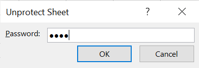
1. Go to the "Review" section. Click on "Unprotect Sheet" option.

2. After completing the above step the below dialog box will open.
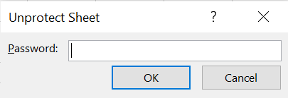
3. Enter the password you provided during protecting the cells.
Now the cells are unprotected.
Step 3: Unhide the formulas
1. Press Ctrl + A to select all the cells of the sheet.

2. Right click and select the "Format cells" option.
3. On the popped-up dialog box, go to "Protection" tab. Uncheck the "Locked" and "Hidden" option to unhide the formulas. Click on "Ok".

Now the formulas are unhidden and unlocked.