Bar graphs are one of the strongest tools in Excel for visualizing and comparing data. Whether we’re tracking sales, analyzing survey responses, or presenting project milestones, bar graphs offer a straightforward way to highlight key trends and differences.
How to Create a Bar Graph in Excel
Here are the steps to create a visually appealing bar graph in Excel to represent our data effectively.
Step 1: Preparing our Data
Ensure our data is organized in a table format. Include one column for categories and one for values.
For Example: In the below data, we have sales of courses.

Step 2: Select ourr Data
- Highlight the entire table, including headers.
- In this case, select cells A1:B7.

Step 3: Insert the Bar Graph
- Go to the Insert tab on the Excel ribbon.
- In the Charts group, click on the Insert Column or Bar Chart icon.
- From the dropdown menu, under 2-D Bar, select Clustered Bar (horizontal bars).
Excel will now insert a bar graph based on ourr selected data.

Step 4: Customize the Bar Graph
1. Add Chart Title
- Click on the default Chart Title at the top of the chart.
- Type a meaningful title, such as "Sales by Product".

2. Add Axis Titles
- Click on the chart to activate the Chart Elements button (the "+" icon on the top-right corner).
- Check the box for Axis Titles.
Add:
- Horizontal Axis Title: Enter "Values" or "Sales" as applicable.
- Vertical Axis Title: Enter "Products" or "Categories".

3. Change Bar Colors
- Click on any bar to select the entire series.
- Right-click and choose Format Data Series.
- Under Fill, choose a new color for the bars.
- To change individual bar colors: Click a specific bar twice > Right-click > Format Data Point > Fill.

4. Add Data Labels
- Right-click on any bar in the graph.
- Select Add Data Labels to display values on the bars.
- Move the labels to ourr preferred position (e.g., inside or outside the bar).

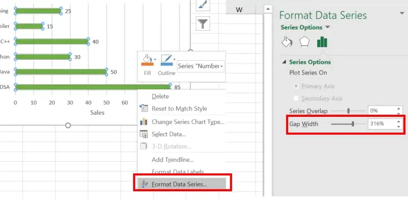
5. Adjust Bar Spacing
- Right-click on any bar and choose Format Data Series.
- Under Series Options, adjust the Gap Width slider to increase or decrease the space between bars.
6. Add or Modify the Legend
- Click on the chart to activate the Chart Elements button (+).
- Check the Legend box to display it.
- Click and drag the legend to position it (e.g., top, right, bottom).

7. Remove Gridlines (Optional)
- Click on any gridline in the chart.
- Press Delete to remove it for a cleaner appearance.
Step 5: Save and Update the Chart
- Save the Excel file to retain ourr changes.
- If our update the data in the table, the bar graph will automatically update.

Types of Bar Graphs in Excel
Excel offers different types of bar graphs to suit ourr needs:
- Clustered Bar Chart: Displays categories side by side for easy comparison.
- Stacked Bar Chart: Bars are stacked on top of each other to show parts of a whole.
- 100% Stacked Bar Chart: Compares the percentage contribution of each category to the whole.
- 3D Bar Chart: Adds a three-dimensional effect to ourr bar graph for a more visual appeal.
Advanced Tips for Bar Graphs
When our make a bar graph in Excel, our can use these advanced tips to enhance its functionality and appearance:
1. Using Secondary Axes for Complex Datasets
- When dealing with data on different scales, add a secondary axis to ourr bar graph.
- Right-click on a data series, choose Format Data Series, and select Secondary Axis to display multiple scales on the same chart.
- This helps compare metrics like sales and profit simultaneously.
2. Combining Bar Graphs with Other Chart Types
- Combine bar graphs with line charts to show trends alongside categorical data.
- Use Combo Chart options in tools like Excel to overlay multiple chart types for enhanced visualization.
- This is especially useful for highlighting relationships between different variables.
3. Exporting Bar Graphs for Presentations
- Copy the chart from ourr tool (e.g., Excel) and paste it directly into Word or PowerPoint using Ctrl + V (Windows) or Cmd + V (Mac).
- For higher quality, save the chart as an image by right-clicking and selecting Save as Picture.
- Resize and adjust the chart in ourr presentation to maintain clarity and visual appeal.
These advanced tips make bar graphs more versatile and presentation-ready for professional use.