Line Chart Visualization in Excel Power View

Line Chart Visualization in Excel Power View is a method used to display data trends over time or across categories using connected data points. It helps users easily compare values, identify patterns, and analyze changes in datasets.

Creating a Visualization

Visualization helps to handle large sets of data by performing drill-up or drill-down operations to extract the essential data. Various visualizations available are listed below:

Table
Map
Matrix
Card
Charts: Line, Bar, bubble, column, scatter

While each of these can be used individually, we can combine all of these charts to provide interactive visualization. For every table or data that we have, we can easily create a visualization that best represents our data. We are going to create a Line chart using Power BI desktop.

Prerequisites:

Excel power view enabled via add-ins, or
Power BI Desktop (for later versions)

Steps for Exploring the Data

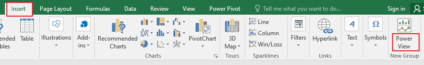
Step 1: Enable Excel Power View by going to Insert -> Power View.

selecting-power-view — Power View button enabled under the “Insert” tab in Excel for creating visual reports.

Step 2: To load the data, go to Data-> Get External Data.

selecting-get-external-data — Data import options displayed while selecting external data sources like Excel, SQL Server, Web, etc.

It will migrate to the dialog box and select "get external data". It will show a list of data sources from which the data could be imported. We can either import from excel, SQL server from the dataset, as text/CSV file, or directly from the web, as a blank query or any template apps.

opening-dataset — Data source selection window showing options like Excel, SQL Server, CSV, Web, and templates.

Step 3: Select any of the data sources. Here we are going to import an access database. Select the file and in the Table import wizard, click on the source table that has data.

select-tables-and-views — Import wizard showing selected table from Access database for use in Power View.

Step 4: It will create a table in excel with the Power View tab as shown below.

table-created — Power View-enabled table loaded into Excel, ready for visualization.

The power view tab helps to create charts and visualization of our data.

Steps to Create a Line Chart

Step 1: Go to the Power View tab.

Step 2: Click on the blank area anywhere and it will open up a power view field on the right-hand side.

power-view-fields — Clicking on a blank area to display the Power View Fields pane on the right

Step 3: Drag and drop the fields in the areas section. Select two fields to be displayed on horizontal (x-axis) and vertical (y-axis) lines. Here we have selected buyer (categorical) data to be displayed on the horizontal line and amount (numerical) displayed on the vertical axis.

selecting-fields — Dragging "Buyer" to X-axis and "Amount" to Y-axis in the field section.

Step 4: In the design tab, go to "change chart type".

Selecting-change-chart-type — Opening the "Change Chart Type" option from the Design tab.

Step 5: Select "Line" from the available options. A blank chart will appear. It will convert a table to a visualization chart.

selecting-line — Choosing "Line" chart from the available chart types.

Step 6: It will generate a line chart as shown below.

line-chart-generated — Line chart generated showing Amount by Buyer.

Filtering with Line Chart Visualization

To filter the data we will first click the actual graph that shows the sum of the amount against various buyers,

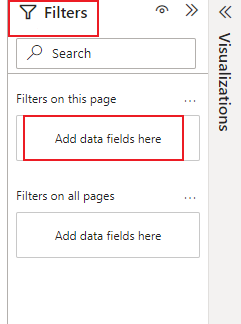
Step 1: Click on the filters pane on the right-hand side. Currently, there are no filters applied so the fields appear blank. Click on the "add data fields here" box.

selecting-add-data-fields-here — Clicking the Filters pane to add a new filter field.

Step 2: We will apply the filter on the "Sum of amount" fields. Go to "show items when value " and select "is less than" among the available selectors. Enter any value (here we have entered 300).

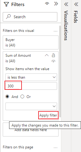
entering-value — Adding "Sum of Amount" field to the filter area.

Step 3: Click on "apply filter" button. A filtered line graph will appear as shown below where the values under the "sum of amount" field will be less than 300.

applying-filter — Filtering data where "Sum of Amount" is less than 300.

Features of Line Chart

The line chart shows the relationship between two values for all items of a table.
Distributes categorical data on the horizontal axis and numerical data on the vertical axis.
Serves perfect analytical representation in 2D for two data item comparisons.
Displays data in chronological order along the vertical axis even if the actual data may not be in the same order or in similar base units.
Great for displaying sequential data or data pertaining to time.